 Indietro
Microeconomics Core Concepts: Utility, Costs, and Perfect Competition
 09:38

Termini in questo insieme (30)
Utility is the satisfaction or benefit a consumer derives from consuming a good or service.
Marginal utility is the additional satisfaction gained from consuming one more unit of a good or service.
MU = change in total utility / change in quantity consumed.
As more units of a good are consumed, the additional satisfaction (marginal utility) from each extra unit decreases.
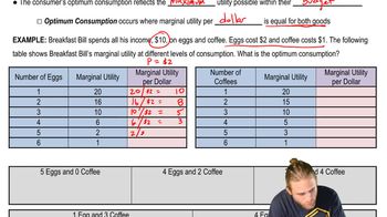
1. The consumer spends all their income.
2. The marginal utility per dollar spent is equal across all goods: \(\frac{MU_x}{P_x} = \frac{MU_y}{P_y}\).
Marginal utility per dollar = marginal utility of the good divided by its price: \(\frac{MU}{P}\).
The change in consumption resulting from a change in purchasing power due to a price change.
The change in consumption resulting from a change in relative prices, causing consumers to substitute toward the relatively cheaper good.
Utility maximization under budget constraints leads consumers to choose quantities that form the basis of individual demand curves.
Explicit costs are direct, out-of-pocket payments for inputs like wages and rent.
Implicit costs are the opportunity costs of using resources owned by the firm, like foregone income.
Economic cost = explicit + implicit costs; Accounting cost = explicit costs only.
Economic profit = total revenue - (explicit costs + implicit costs).
Short run: at least one input is fixed.
Long run: all inputs can vary.
Fixed costs do not change with output (e.g., rent).
Variable costs change with output (e.g., labor).
The additional output produced by adding one more unit of labor.
As more labor is added, the MPL eventually decreases.
Total cost = fixed costs + variable costs.
AFC = fixed cost / quantity.
AVC = variable cost / quantity.
ATC = total cost / quantity.
MC is the additional cost of producing one more unit of output.
Marginal cost pulls average costs: when MC < ATC, ATC falls; when MC > ATC, ATC rises.
It shows the lowest possible average cost when all inputs can vary, representing the planning horizon.
MES is the smallest output level at which long run average cost is minimized.
Economies of scale: average costs decrease as output increases.
Diseconomies of scale: average costs increase as output increases.
Many buyers and sellers, identical products, free entry and exit, and perfect information.
The firm faces a perfectly elastic demand curve at the market price.
Produce where marginal revenue equals marginal cost: \(MR = MC\). Since \(P = MR\), set \(P = MC\).
Shut down if price is less than minimum average variable cost: \(P < AVC_{min}\).
Entry and exit drive economic profits to zero, leading to long run competitive equilibrium.
Because firms produce at minimum average cost and price equals marginal cost, maximizing total surplus.