Ch. 8 - Integration Techniques
Briggs - Calculus: Early Transcendentals 3rd Edition
Briggs3rd EditionCalculus: Early TranscendentalsISBN: 9780136847243Non è quello che usi tu?Cambia libro di testo
Capitolo 8, Problema 8.8.15

15-18. {Use of Tech} Midpoint Rule approximations. Find the indicated Midpoint Rule approximations to the following integrals.
15. ∫(2 to 10) 2x² dx using n = 1, 2, and 4 subintervals

Guida verificata passo dopo passo
1
Step 1: Understand the Midpoint Rule. The Midpoint Rule is a numerical method to approximate the value of a definite integral. It divides the interval into 'n' subintervals, calculates the midpoint of each subinterval, evaluates the function at these midpoints, and then multiplies by the width of the subintervals.
Step 2: Identify the integral and interval. The integral is ∫(2 to 10) 2x² dx, and the interval is [2, 10]. The number of subintervals (n) will vary as specified: n = 1, n = 2, and n = 4.
Step 3: Calculate the width of each subinterval (Δx). The formula for Δx is Δx = (b - a) / n, where 'a' is the lower limit (2), 'b' is the upper limit (10), and 'n' is the number of subintervals. Compute Δx for n = 1, n = 2, and n = 4.
Step 4: Determine the midpoints of each subinterval. For each subinterval, the midpoint is calculated as (x_i + x_(i+1)) / 2, where x_i and x_(i+1) are the endpoints of the subinterval. Compute the midpoints for n = 1, n = 2, and n = 4.
Step 5: Apply the Midpoint Rule formula. The approximation is given by M_n = Δx * Σ[f(midpoint_i)], where f(x) = 2x² is the function being integrated, Δx is the width of the subintervals, and midpoint_i are the midpoints of the subintervals. Evaluate the sum for n = 1, n = 2, and n = 4.

Risposta video verificata per un problema simile:

Questa soluzione video è stata consigliata dai nostri tutor come utile per risolvere questo problema.
Durata del video:
2m

Concetti chiave

Ecco i concetti essenziali che devi comprendere per rispondere correttamente alla domanda.

Midpoint Rule

The Midpoint Rule is a numerical method used to approximate the value of a definite integral. It involves dividing the interval of integration into subintervals, calculating the midpoint of each subinterval, and then evaluating the function at these midpoints. The area under the curve is then approximated by summing the areas of rectangles formed by these midpoints, multiplied by the width of the subintervals.
Video consigliato:
Percorso guidato
07:39
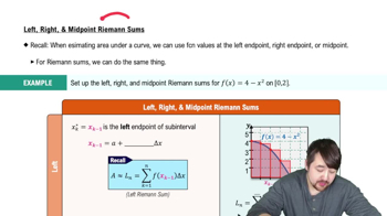
Left, Right, & Midpoint Riemann Sums

Definite Integral

A definite integral represents the signed area under a curve defined by a function over a specific interval [a, b]. It is denoted as ∫(a to b) f(x) dx and provides a way to calculate total accumulation, such as area, volume, or other quantities. The Fundamental Theorem of Calculus connects the concept of differentiation with integration, allowing for the evaluation of definite integrals using antiderivatives.
Video consigliato:
Percorso guidato
05:43
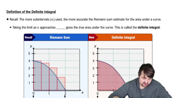
Definition of the Definite Integral

Subintervals

Subintervals are smaller segments into which the main interval of integration is divided when applying numerical methods like the Midpoint Rule. The number of subintervals, denoted as 'n', affects the accuracy of the approximation; more subintervals generally lead to a better approximation of the integral. Each subinterval has a width calculated as (b - a) / n, where [a, b] is the interval of integration.
Video consigliato:
Percorso guidato
06:11
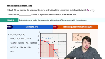
Introduction to Riemann Sums