Ch. 9 - First-Order Differential Equations
Hass - Thomas' Calculus 15th Edition
Hass15th EditionThomas' CalculusISBN: 9780137616077Non è quello che usi tu?Cambia libro di testo
Capitolo 9, Problema 9.2.15

Solving Initial Value Problems
Solve the initial value problems in Exercises 15–20.
dy/dt + 2y = 3, y(0) = 1

Guida verificata passo dopo passo
1
Identify the type of differential equation. The given equation is a first-order linear ordinary differential equation of the form \(\frac{dy}{dt} + P(t)y = Q(t)\), where \(P(t) = 2\) and \(Q(t) = 3\).
Find the integrating factor \(\mu(t)\) using the formula \(\mu(t) = e^{\int P(t)\,dt}\). In this case, calculate \(\mu(t) = e^{\int 2\,dt}\).
Multiply both sides of the differential equation by the integrating factor \(\mu(t)\) to rewrite the left side as the derivative of a product: \(\frac{d}{dt}[\mu(t) y] = \mu(t) Q(t)\).
Integrate both sides with respect to \(t\) to find \(\mu(t) y = \int \mu(t) Q(t)\, dt + C\), where \(C\) is the constant of integration.
Use the initial condition \(y(0) = 1\) to solve for the constant \(C\), then solve for \(y(t)\) by dividing both sides by \(\mu(t)\).

Risposta video verificata per un problema simile:

Questa soluzione video è stata consigliata dai nostri tutor come utile per risolvere questo problema.
Durata del video:
3m

Concetti chiave

Ecco i concetti essenziali che devi comprendere per rispondere correttamente alla domanda.

First-Order Linear Differential Equations

These are differential equations of the form dy/dt + P(t)y = Q(t), where the solution involves finding an integrating factor to simplify the equation. Recognizing this form allows the use of systematic methods to solve for y(t).
Video consigliato:
07:39
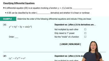
Classifying Differential Equations

Integrating Factor Method

This technique involves multiplying the entire differential equation by an integrating factor, usually e^(∫P(t)dt), to rewrite the left side as a derivative of a product. This simplifies solving the equation by enabling direct integration.
Video consigliato:
07:33
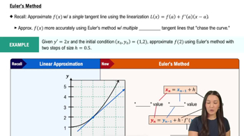
Euler's Method

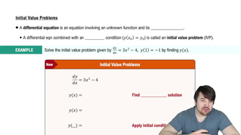
Initial Value Problems (IVP)

An IVP specifies the value of the unknown function at a particular point, such as y(0) = 1. This condition is used to find the unique solution to the differential equation that satisfies the initial condition.
Video consigliato:
Percorso guidato
05:03
Initial Value Problems