 Indietro
Introductory Statistics Key Concepts
 04:52
04:52
Termini in questo insieme (20)
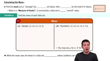
The population mean \(\mu\) is calculated as the sum of all values divided by the population size: \(\mu = \frac{\sum_{i=1}^N x_i}{N}\).
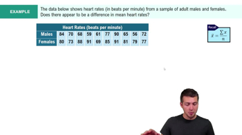
The sample mean \(\bar{x}\) is the sum of all sample values divided by the sample size: \(\bar{x} = \frac{\sum_{i=1}^n x_i}{n}\).
Population variance \(\sigma^2\) is the average of squared differences from the mean: \(\sigma^2 = \frac{\sum_{i=1}^N (x_i - \mu)^2}{N}\).
Sample variance \(s^2\) is the adjusted average of squared differences from the sample mean: \(s^2 = \frac{\sum_{i=1}^n (x_i - \bar{x})^2}{n-1}\).
Standard deviation is the square root of the variance, providing a measure of spread in the same units as the data.
Skewness measures the asymmetry of a distribution around the mean: zero skewness is symmetric, positive skewness indicates a right tail, and negative skewness indicates a left tail.
A symmetric distribution has skewness = 0, and the mean equals the median.
Moderately right skewed distributions have skewness > 0, with the mean usually greater than the median.
Moderately left skewed distributions have skewness < 0, with the mean usually less than the median.
Kurtosis measures the heaviness of a distribution's tails relative to its center, indicating the likelihood of extreme values.
Leptokurtic: kurtosis > 3 (heavy tails), Mesokurtic: kurtosis = 3 (normal), Platykurtic: kurtosis < 3 (light tails).
A box plot graphically displays the five-number summary: minimum, Q1, median, Q3, and maximum, highlighting data spread and outliers.
Approximately 68% of data lie within 1 standard deviation, 95% within 2, and 99.7% within 3 standard deviations of the mean.
A normal distribution with mean 0 and standard deviation 1, used to calculate probabilities for standardized values (z-scores).
A z-score indicates how many standard deviations a value is from the mean: z=0 at mean, z>0 above mean, z<0 below mean.
\(z = \frac{\bar{x} - \mu}{\sigma / \sqrt{n}}\), where \(\bar{x}\) is sample mean, \(\mu\) population mean, \(\sigma\) population standard deviation, and \(n\) sample size.
The sampling distribution of the sample mean is approximately normal if the population is normal or the sample size is large (usually n>30).
Standard error = \(\frac{\sigma}{\sqrt{n}}\), where \(\sigma\) is population standard deviation and \(n\) is sample size.
Fixed number of independent trials, two outcomes per trial (success/failure), constant probability of success \(\pi\), and the random variable counts number of successes.
When both \(n\pi \geq 10\) and \(n(1-\pi) \geq 10\) are satisfied, the binomial distribution is approximately normal.