 Indietro
Introductory Statistics: Probability Distributions and Discrete Distributions
 04:14
04:14
Termini in questo insieme (20)
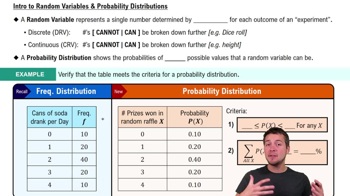
A random variable represents a numerical value associated with each outcome of a probability distribution, denoted by \(x\).
A discrete random variable has a finite or countable number of possible outcomes that can be listed.
A continuous random variable has an uncountable number of possible outcomes, represented by an interval on the number line.
It is discrete because the number of companies can be counted.
It is continuous because the volume can be any value between 0 and 21 gallons.
1) Each probability is between 0 and 1 inclusive: \(0 \leq P(x) \leq 1\).
2) The sum of all probabilities is 1: \(\sum P(x) = 1\).
Make a frequency distribution, sum frequencies, find probabilities by dividing each frequency by the total, and verify probabilities sum to 1 and are between 0 and 1.
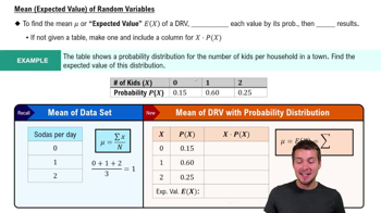
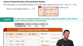
The mean \(\mu\) is the sum of each value multiplied by its probability: \(\mu = \sum xP(x)\).
Variance \(\sigma^2\) is \(\sigma^2 = \sum (x - \mu)^2 P(x)\).
Standard deviation \(\sigma\) is the square root of the variance: \(\sigma = \sqrt{\sigma^2} = \sqrt{\sum (x - \mu)^2 P(x)}\).
The expected value is equal to the mean: \(E(x) = \mu = \sum xP(x)\).
1) Fixed number of independent trials.
2) Two possible outcomes per trial (success or failure).
3) Constant probability of success \(p\).
4) Random variable \(x\) counts number of successes.
\(P(x) = \binom{n}{x} p^x q^{n-x}\), where \(q = 1 - p\).
The mean is \(\mu = np\), where \(n\) is trials and \(p\) is success probability.
Variance is \(\sigma^2 = npq\), where \(q = 1 - p\).
Standard deviation is \(\sigma = \sqrt{npq}\).
A geometric distribution models the number of trials until the first success, with independent trials and constant success probability \(p\).
\(P(x) = p q^{x-1}\), where \(q = 1 - p\) and \(x\) is the trial of first success.
The Poisson distribution models the number of times an event occurs in a fixed interval, with independent occurrences and constant average rate \(\mu\).
\(P(x) = \frac{\mu^x e^{-\mu}}{x!}\), where \(e \approx 2.71818\) and \(\mu\) is the mean number of occurrences.