Ch. 2 - Descriptive Statistics
Larson - Elementary Statistics: Picturing the World 8th Edition
Larson8th EditionElementary Statistics: Picturing the WorldISBN: 9780137493470Non è quello che usi tu?Cambia libro di testo
Capitolo 2, Problema 2.1.20d

Use the frequency histogram
describe any patterns with the data..
A frequency histogram showing roller coaster heights in feet, with the highest frequency at 125 feet.

Guida verificata passo dopo passo
1
Step 1: Observe the histogram and identify the key components. The x-axis represents the height of roller coasters (in feet), divided into intervals, while the y-axis represents the frequency (number of roller coasters) within each height interval.
Step 2: Note the distribution of the data. The histogram shows that the majority of roller coasters fall within the height range of 125 to 178 feet, as this interval has the highest frequency (approximately 40).
Step 3: Identify any patterns or trends. The data appears to be skewed to the right, as the frequency decreases for higher height intervals (231-284 feet and beyond). This suggests that taller roller coasters are less common.
Step 4: Consider the spread of the data. The heights range from 72 feet to 337 feet, indicating a wide variety of roller coaster heights. However, most roller coasters are concentrated in the lower height intervals.
Step 5: Summarize the findings. The histogram indicates that roller coasters are most commonly built within the height range of 125 to 178 feet, with fewer roller coasters at extreme heights. This could reflect design or safety considerations in roller coaster construction.

Risposta video verificata per un problema simile:

Questa soluzione video è stata consigliata dai nostri tutor come utile per risolvere questo problema.
Durata del video:
2m

Concetti chiave

Ecco i concetti essenziali che devi comprendere per rispondere correttamente alla domanda.

Frequency Histogram

A frequency histogram is a graphical representation of data that shows the frequency of data points within specified ranges, or bins. Each bar's height indicates the number of observations that fall within that range, allowing for a visual interpretation of the distribution of the data. In this case, the histogram displays the heights of roller coasters, making it easy to identify which height ranges are most common.
Video consigliato:
Percorso guidato
05:54
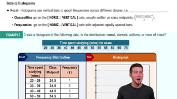
Intro to Histograms

Central Tendency

Central tendency refers to the statistical measures that describe the center of a data set, commonly represented by the mean, median, and mode. In the context of the histogram, the mode is particularly relevant as it indicates the height range with the highest frequency, which is 125 feet in this case. Understanding central tendency helps in summarizing the data and identifying typical values.
Video consigliato:
Percorso guidato
04:52
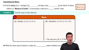
Calculating the Mean

Data Distribution Patterns

Data distribution patterns refer to the way data points are spread across different values, which can reveal trends, clusters, or gaps in the data. Analyzing the histogram can help identify whether the data is normally distributed, skewed, or has outliers. In this histogram, the concentration of roller coasters around 125 feet suggests a common height preference, while the tapering off at higher heights indicates fewer roller coasters at those elevations.
Video consigliato:
Percorso guidato
04:39
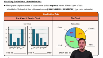
Visualizing Qualitative vs. Quantitative Data
Pratica correlata
Domanda del libro di testo

Extending Concepts


Golf The distances (in yards) for nine holes of a golf course are listed.

336 393 408 522 147 504 177 375 360


d. Use your results from part (c) to explain how to quickly find the mean and the median of the original data set when the distances are converted to inches.

95
views
Domanda del libro di testo

Using and Interpreting Concepts


Using and Interpreting Concepts Finding Quartiles, Interquartile Range, and Outliers In Exercises 11 and 12,

(c) identify any outliers.


56 63 51 60 57 60 60 54 63 59 80 63 60 62 65

148
views
Domanda del libro di testo

Song Lengths Side-by-side box-and-whisker plots can be used to compare two or more different data sets. Each box-and-whisker plot is drawn on the same number line to compare the data sets more easily. The lengths (in seconds) of songs played at two different concerts are shown.

d. Can you determine which concert lasted longer? Explain.

121
views
Domanda del libro di testo

Use the frequency histogram

d. describe any patterns with the data..

158
views
Domanda del libro di testo

Studying Refer to the data set in Exercise 23 and the box-and-whisker plot you drew that represents the data set.


c. You randomly select one student from the sample. What is the likelihood that the student studied less than 2 hours per day? Write your answer as a percent.

94
views
Domanda del libro di testo

Pearson’s Index of Skewness The English statistician Karl Pearson (1857–1936) introduced a formula for the skewness of a distribution.

P = 3 (x̄ - median) / s

Most distributions have an index of skewness between -3 and 3. When P > 0, the data are skewed right. When P < 0, the data are skewed left. When P = 0, the data are symmetric. Calculate the coefficient of skewness for each distribution. Describe the shape of each.


c. x̄ = 9.2, s = 1.8, median = 9.2

529
views