Car Colors
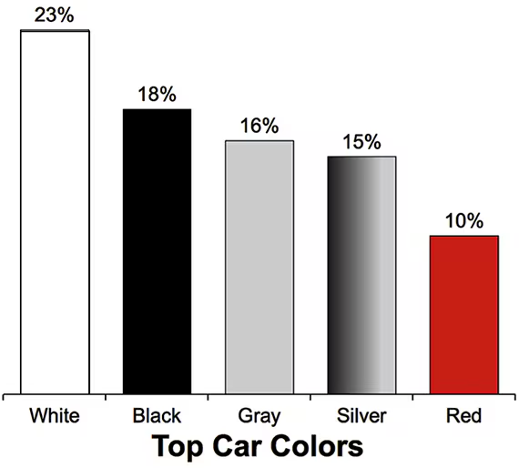
In Exercises 9–12, assume that 100 cars are randomly selected. Refer to the accompanying graph, which shows the top car colors and the percentages of cars with those colors (based on PPG Industries).





Black Cars Find the probability that at least 25 cars are black. Is 25 a significantly high number of black cars?

Standard Normal Distribution. In Exercises 13–16, find the indicated z score. The graph depicts the standard normal distribution of bone density scores with mean 0 and standard deviation 1.

Outliers For the purposes of constructing modified boxplots as described in Section 3-3, outliers are defined as data values that are above Q3 by an amount greater than 1.5 x IQR or below Q1 by an amount greater than 1.5 x IQR, where IQR is the interquartile range. Using this definition of outliers, find the probability that when a value is randomly selected from a normal distribution, it is an outlier.

Determining Normality. In Exercises 9–12, refer to the indicated sample data and determine whether they appear to be from a population with a normal distribution. Assume that this requirement is loose in the sense that the population distribution need not be exactly normal, but it must be a distribution that is roughly bell-shaped.

Taxi Trips The distances (miles) traveled by New York City taxis transporting customers, as listed in Data Set 32 “Taxis” in Appendix B

Standard Normal Distribution. In Exercises 17–36, assume that a randomly selected subject is given a bone density test. Those test scores are normally distributed with a mean of 0 and a standard deviation of 1. In each case, draw a graph, then find the probability of the given bone density test scores. If using technology instead of Table A-2, round answers to four decimal places.

Between 1.50 and 2.00

Constructing Normal Quantile Plots. In Exercises 17–20, use the given data values to identify the corresponding z scores that are used for a normal quantile plot, then identify the coordinates of each point in the normal quantile plot. Construct the normal quantile plot, then determine whether the data appear to be from a population with a normal distribution.

Earthquake Depths A sample of depths (km) of earthquakes is obtained from Data Set 24 “Earthquakes” in Appendix B: 17.3, 7.0, 7.0, 7.0, 8.1, 6.8.

Finding Bone Density Scores. In Exercises 37–40 assume that a randomly selected subject is given a bone density test. Bone density test scores are normally distributed with a mean of 0 and a standard deviation of 1. In each case, draw a graph, then find the bone density test score corresponding to the given information. Round results to two decimal places.

Find P99, the 99th percentile. This is the bone density score separating the bottom 99% from the top 1%.