Ch 26: Potential and Field
Knight Calc - Physics for Scientists and Engineers 5th Edition
Knight Calc5th EditionPhysics for Scientists and EngineersISBN: 9780137344796당신이 사용하는 게 아니라요?교과서 변경
26장, 문제 39a

The electric field in a region of space is Ex = −1000x^2 V/m, where x is in meters. Graph Ex versus x over the region −1 m ≤ x ≤1 m.

검증된 단계별 안내
1
Understand the given electric field expression: The electric field is given as \( E_x = -1000x^2 \) V/m, where \( x \) is the position in meters. This means the electric field depends on the square of \( x \), and it is negative, indicating direction.
Identify the range for \( x \): The problem specifies the range \( -1 \leq x \leq 1 \) meters. This will be the domain for the graph.
Determine the behavior of \( E_x \): Since \( E_x = -1000x^2 \), the electric field is always negative (due to the \( -1000 \) factor) and symmetric about \( x = 0 \) because \( x^2 \) is an even function. The maximum magnitude of \( E_x \) occurs at \( x = \pm 1 \).
Calculate key points for the graph: Evaluate \( E_x \) at specific values of \( x \) within the range, such as \( x = -1, -0.5, 0, 0.5, 1 \). For example, at \( x = 0 \), \( E_x = -1000(0)^2 = 0 \); at \( x = 1 \), \( E_x = -1000(1)^2 = -1000 \) V/m.
Plot the graph: On the horizontal axis, represent \( x \) from \( -1 \) to \( 1 \). On the vertical axis, represent \( E_x \) values. Plot the calculated points and connect them with a smooth curve, showing a parabolic shape opening downward (negative values) and symmetric about \( x = 0 \).

비슷한 문제에 대한 검증된 영상 답변:

이 영상 해법은 위 문제에 도움이 된다고 튜터들이 추천한 것입니다.
영상 길이:
3m

주요 개념

질문에 올바르게 답하기 위해 반드시 이해해야 하는 핵심 개념들은 다음과 같습니다.

Electric Field

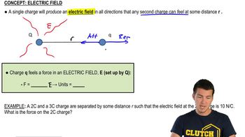
The electric field is a vector field that represents the force per unit charge experienced by a positive test charge placed in the field. It is defined mathematically as E = F/q, where E is the electric field, F is the force, and q is the charge. In this case, the electric field varies with position, specifically as a function of x, indicating how the force changes as the position changes.
추천 영상:
가이드 코스
03:16
Intro to Electric Fields

Graphing Functions

Graphing functions involves plotting points on a coordinate system to visualize the relationship between variables. In this context, we are graphing the electric field Ex as a function of position x. Understanding how to interpret the graph helps in analyzing the behavior of the electric field across the specified range, revealing trends such as symmetry and the nature of the field's variation.
추천 영상:
가이드 코스
08:30
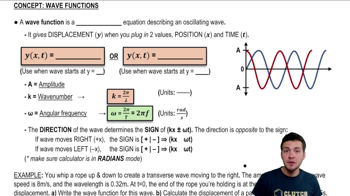
Intro to Wave Functions

Quadratic Functions

A quadratic function is a polynomial function of degree two, typically expressed in the form f(x) = ax^2 + bx + c. The given electric field Ex = -1000x^2 V/m is a quadratic function where the coefficient of x^2 is negative, indicating that the graph will be a downward-opening parabola. Recognizing the characteristics of quadratic functions is essential for accurately graphing and interpreting the electric field's behavior.
추천 영상:
가이드 코스
5:13
Quadratic Equations