Ch. 9 - Differential Equations
Briggs - Calculus: Early Transcendentals 3rd Edition
Briggs3rd EditionCalculus: Early TranscendentalsISBN: 9780136847243당신이 사용하는 게 아니라요?교과서 변경
9장, 문제 9.5.15

15–16. {Use of Tech} Solving logistic equations Write a logistic equation with the following parameter values. Then solve the initial value problem and graph the solution. Let r be the natural growth rate, K the carrying capacity, and P₀ the initial population.


r=0.2, K=300, P₀=50

검증된 단계별 안내
1
Start by writing the general form of the logistic differential equation: \[\frac{dP}{dt} = rP\left(1 - \frac{P}{K}\right)\] where \(P(t)\) is the population at time \(t\), \(r\) is the natural growth rate, and \(K\) is the carrying capacity.
Substitute the given parameter values into the logistic equation: \[\frac{dP}{dt} = 0.2P\left(1 - \frac{P}{300}\right)\].
Set up the initial value problem (IVP) by including the initial condition: \[P(0) = 50\].
To solve the IVP, separate variables and integrate: rewrite the equation as \[\frac{dP}{P(1 - P/300)} = 0.2\,dt\] and then perform partial fraction decomposition on the left side before integrating both sides.
After integrating, solve for \(P(t)\) explicitly in terms of \(t\) and the constants, then use the initial condition \(P(0) = 50\) to find the constant of integration. This will give you the logistic growth function describing the population over time.

비슷한 문제에 대한 검증된 영상 답변:

이 영상 해법은 위 문제에 도움이 된다고 튜터들이 추천한 것입니다.
영상 길이:
8m
도움이 되었나요?

주요 개념

질문에 올바르게 답하기 위해 반드시 이해해야 하는 핵심 개념들은 다음과 같습니다.

Logistic Growth Model

The logistic growth model describes population growth that starts exponentially but slows as the population approaches a maximum limit called the carrying capacity (K). It is represented by the differential equation dP/dt = rP(1 - P/K), where r is the natural growth rate and P is the population at time t.
추천 영상:
09:29
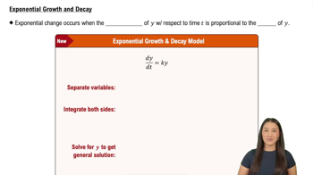
Exponential Growth & Decay

Solving Initial Value Problems (IVPs)

An initial value problem involves solving a differential equation with a given initial condition, such as P(0) = P₀. Solving the logistic equation IVP means finding a function P(t) that satisfies both the logistic differential equation and the initial population value.
추천 영상:
05:03
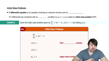
Initial Value Problems

Graphing Solutions of Differential Equations

Graphing the solution to a logistic equation shows how the population changes over time, typically starting at P₀, growing rapidly, and leveling off near the carrying capacity K. This visual helps interpret the behavior and stability of the population model.
추천 영상:
04:00
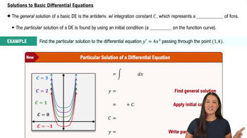
Solutions to Basic Differential Equations