Ch. 9 - Differential Equations
Briggs - Calculus: Early Transcendentals 3rd Edition
Briggs3rd EditionCalculus: Early TranscendentalsISBN: 9780136847243당신이 사용하는 게 아니라요?교과서 변경
9장, 문제 9.5.27e

27–30. Predator-prey models Consider the following pairs of differential equations that model a predator-prey system with populations x and y. In each case, carry out the following steps.


e. Sketch a representative solution curve in the xy-plane and indicate the direction in which the solution evolves.


x′(t) = −3x + 6xy, y′(t) = y − 4xy

검증된 단계별 안내
1
Identify the system of differential equations given: \(x'(t) = -3x + 6xy\) and \(y'(t) = y - 4xy\). Here, \(x(t)\) and \(y(t)\) represent the populations of prey and predator, respectively.
Find the equilibrium points by setting \(x'(t) = 0\) and \(y'(t) = 0\). Solve the system of algebraic equations: \(-3x + 6xy = 0\) and \(y - 4xy = 0\) to find points where the populations do not change.
Analyze the direction of the vector field around the equilibrium points by considering the signs of \(x'(t)\) and \(y'(t)\) in different regions of the \(xy\)-plane. This helps determine how the populations evolve over time near these points.
Sketch the nullclines: curves where \(x'(t) = 0\) and \(y'(t) = 0\). These nullclines divide the plane into regions where the direction of change of \(x\) and \(y\) can be determined, guiding the shape of the solution trajectories.
Draw representative solution curves in the \(xy\)-plane by following the direction of the vector field, starting from various initial points. Indicate the direction of time evolution with arrows along the curves to show how the populations change.

비슷한 문제에 대한 검증된 영상 답변:

이 영상 해법은 위 문제에 도움이 된다고 튜터들이 추천한 것입니다.
영상 길이:
3m
도움이 되었나요?

주요 개념

질문에 올바르게 답하기 위해 반드시 이해해야 하는 핵심 개념들은 다음과 같습니다.

Predator-Prey Differential Equations

Predator-prey models use coupled differential equations to describe interactions between two species: prey (x) and predator (y). The equations capture growth and decline rates influenced by each population, reflecting biological interactions such as predation and reproduction.
추천 영상:
07:39
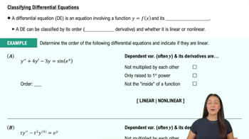
Classifying Differential Equations

Phase Plane and Solution Curves

The phase plane is a graphical representation where each point corresponds to a state (x, y) of the system. Solution curves trace the trajectory of populations over time, showing how the system evolves. Sketching these curves helps visualize dynamics and stability.
추천 영상:
가이드 코스
06:49
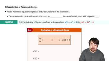
Differentiation of Parametric Curves

Direction Fields and Vector Fields

Direction fields assign a vector to each point in the phase plane, indicating the instantaneous direction of the system's evolution. They guide the drawing of solution curves and show whether populations increase or decrease, helping to understand the flow of the system.
추천 영상:
05:45
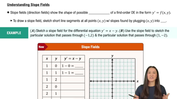
Understanding Slope Fields