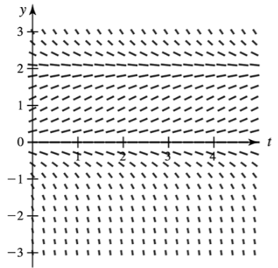
Direction fields Consider the direction field for the equation y′=y(2−y) shown in the figure and initial conditions of the form y(0)=A.
a. Sketch a solution on the direction field with the initial condition y(0)=1.

검증된 단계별 안내

Identify the differential equation given: \(y' = y(2 - y)\). This tells us the slope of the solution curve at any point \((t, y)\) depends on the value of \(y\) at that point.

Note the initial condition \(y(0) = 1\). This means the solution curve must pass through the point \((0, 1)\) on the \(t\)-\(y\) plane.

Examine the direction field at \(y = 1\). Calculate the slope at this point using the differential equation: \(y' = 1 \times (2 - 1) = 1\). So, the slope of the solution curve at \(t=0\) and \(y=1\) is 1.

Using the slope from the direction field at \((0,1)\), sketch a curve starting at this point that follows the slope vectors shown in the direction field. The curve should move upward initially since the slope is positive.

Observe the behavior of the solution as \(t\) increases. Since \(y' = y(2 - y)\), when \(y\) approaches 2, the slope \(y'\) approaches zero, indicating the solution curve will level off near \(y=2\). Sketch the curve approaching this horizontal asymptote as \(t\) grows.

비슷한 문제에 대한 검증된 영상 답변:

이 영상 해법은 위 문제에 도움이 된다고 튜터들이 추천한 것입니다.

영상 길이:

도움이 되었나요?

주요 개념

질문에 올바르게 답하기 위해 반드시 이해해야 하는 핵심 개념들은 다음과 같습니다.

Direction Fields

A direction field is a graphical representation of a first-order differential equation showing slope vectors at various points. Each small line segment indicates the slope of the solution curve passing through that point, helping visualize the behavior of solutions without solving the equation explicitly.

Autonomous Differential Equations

An autonomous differential equation has the form y' = f(y), where the rate of change depends only on y, not on the independent variable t. This allows for analysis of equilibrium points and stability by examining where f(y) = 0, which correspond to constant solutions.

Equilibrium Solutions and Stability

Equilibrium solutions occur where y' = 0, meaning the solution remains constant. Stability depends on the sign of the derivative of f(y) at these points: if small perturbations decay over time, the equilibrium is stable; if they grow, it is unstable. This helps predict long-term behavior of solutions.

Direction fields Consider the direction field for the equation y′=y(2−y) shown in the figure and initial conditions of the form y(0)=A. a. Sketch a solution on the direction field with the initial condition y(0)=1.