Ch. 10 - Chi-Square Tests and the F-Distribution
Larson - Elementary Statistics: Picturing the World 8th Edition
Larson8th EditionElementary Statistics: Picturing the WorldISBN: 9780137493470당신이 사용하는 게 아니라요?교과서 변경
10장, 문제 10.RE.3

In Exercises 1–4, (a) identify the claim and state H₀ and Hₐ, (b) find the critical value and identify the rejection region, (c) find the chi-square test statistic, (d) decide whether to reject or fail to reject the null hypothesis, and (e) interpret the decision in the context of the original claim.


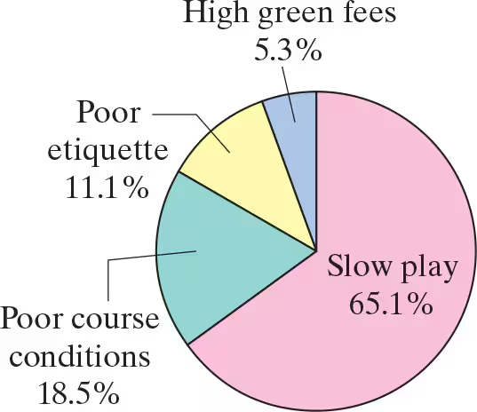
A sports website claims that the opinions of golfers about what irritates them the most on the golf course are distributed as shown in the pie chart. You randomly select 1018 golfers and ask them what irritates them the most on the golf course. The table shows the results. At α=0.05, test the sports website’s claim. (Adapted from GOLF.com)


Pie chart showing golfer irritations: Slow play 65.1%, Poor course conditions 18.5%, Poor etiquette 11.1%, High green fees 5.3%.

검증된 단계별 안내
1
Step 1: Identify the claim and state the null hypothesis (H₀) and alternative hypothesis (Hₐ). The claim is that the opinions of golfers about what irritates them the most on the golf course are distributed as shown in the pie chart: Slow play (65.1%), Poor course conditions (18.5%), Poor etiquette (11.1%), High green fees (5.3%). H₀: The observed frequencies match the claimed distribution. Hₐ: The observed frequencies do not match the claimed distribution.
Step 2: Calculate the expected frequencies for each category based on the claimed percentages and the total sample size of 1018 golfers. Use the formula: Expected frequency = (Percentage / 100) × Total sample size. For example, for Slow play: Expected frequency = (65.1 / 100) × 1018.
Step 3: Compute the chi-square test statistic using the formula: χ² = Σ((Observed frequency - Expected frequency)² / Expected frequency). For each category (Slow play, Poor course conditions, Poor etiquette, High green fees), calculate the contribution to the chi-square statistic and sum them up.
Step 4: Determine the critical value and rejection region for the chi-square test. Use the chi-square distribution table with degrees of freedom (df = number of categories - 1). Here, df = 4 - 1 = 3. At α = 0.05, find the critical value corresponding to df = 3.
Step 5: Compare the calculated chi-square test statistic to the critical value. If the test statistic exceeds the critical value, reject the null hypothesis (H₀). Otherwise, fail to reject H₀. Interpret the decision in the context of the original claim: If H₀ is rejected, the observed frequencies do not match the claimed distribution; if H₀ is not rejected, the observed frequencies are consistent with the claimed distribution.

비슷한 문제에 대한 검증된 영상 답변:

이 영상 해법은 위 문제에 도움이 된다고 튜터들이 추천한 것입니다.
영상 길이:
6m

주요 개념

질문에 올바르게 답하기 위해 반드시 이해해야 하는 핵심 개념들은 다음과 같습니다.

Hypothesis Testing

Hypothesis testing is a statistical method used to make decisions about a population based on sample data. It involves formulating two competing hypotheses: the null hypothesis (H₀), which represents a statement of no effect or no difference, and the alternative hypothesis (Hₐ), which indicates the presence of an effect or difference. The goal is to determine whether there is enough evidence in the sample data to reject H₀ in favor of Hₐ.
추천 영상:
가이드 코스
06:21
Step 1: Write Hypotheses

Chi-Square Test

The chi-square test is a statistical test used to determine if there is a significant association between categorical variables. It compares the observed frequencies in each category to the expected frequencies under the null hypothesis. The test statistic follows a chi-square distribution, and the critical value is determined based on the desired significance level (α) and the degrees of freedom, which is calculated from the number of categories.
추천 영상:
가이드 코스
07:01
Intro to Least Squares Regression

Rejection Region

The rejection region is the range of values for the test statistic that leads to the rejection of the null hypothesis. It is determined by the significance level (α) and the critical value from the chi-square distribution. If the calculated test statistic falls within this region, it suggests that the observed data is unlikely under the null hypothesis, prompting researchers to reject H₀ and accept Hₐ, thereby supporting the alternative claim.
추천 영상:
가이드 코스
09:56
Step 4: State Conclusion
관련 실천
교과서 질문

In Exercises 9–12, find the critical F-value for a right-tailed test using the level of significance α and degrees of freedom d.f.N and d.f.D.


α=0.05,d.f.N=20,d.f.D=25

79
views

교과서 질문

In Exercises 13–16, find the critical F-value for a two-tailed test using the level of significance α and degrees of freedom d.f.N and d.f.D.


α=0.01,d.f.N=11,d.f.D=13

58
views
교과서 질문

In each exercise,

d. decide whether to reject or fail to reject the null hypothesis, and

[APPLET] In Exercises 1–3, use the data, which list the hourly wages (in dollars) for randomly selected surgical technologists from three states. Assume the wages are normally distributed and that the samples are independent. (Adapted from U.S. Bureau of Labor Statistics)

Maine: 22.76, 27.60, 25.08, 17.01, 30.15, 27.09, 20.95, 25.52, 20.11, 23.67, 24.32

Oklahoma: 24.64, 21.66, 19.38, 18.19, 23.14, 20.58, 19.53, 30.77, 27.46, 23.80

Massachusetts: 27.07, 24.71, 32.80, 28.34, 33.45, 33.36, 36.81, 30.04, 29.01, 24.30, 29.22, 29.50

Are the mean hourly wages of surgical technologists the same for all three states? Use α=0.01. Assume that the population variances are equal.

21
views
교과서 질문

"In Exercises 9–12, find the critical F-value for a right-tailed test using the level of significance α and degrees of freedom d.f.N and d.f.D.


α=0.01,d.f.N=12,d.f.D=10"

53
views
교과서 질문

In Exercises 5–8, (a) find the expected frequency for each cell in the contingency table, (b) identify the claim and state H0 and Ha, (c) determine the degrees of freedom, find the critical value, and identify the rejection region, (d) find the chi-square test statistic, (e) decide whether to reject or fail to reject the null hypothesis, and (f) interpret the decision in the context of the original claim.


The contingency table shows the distribution of a random sample of fatal pedestrian and bicyclist motor vehicle collisions by time of day in a recent year. At α=0.10, can you conclude that the type of crash victim and the time of day are related? (Adapted from National Highway Traffic Safety Administration)


106
views
교과서 질문

In Exercises 13–16, find the critical F-value for a two-tailed test using the level of significance α and degrees of freedom d.f.N and d.f.D.


α=0.01,d.f.N=40,d.f.D=60

63
views