Ch. 8 - Hypothesis Testing with Two Samples

Larson - Elementary Statistics: Picturing the World 8th Edition

Larson8th EditionElementary Statistics: Picturing the WorldISBN: 9780137493470당신이 사용하는 게 아니라요?교과서 변경

Larson 8th Edition

Ch. 8 - Hypothesis Testing with Two Samples

문제 8.2.22

8장, 문제 8.2.22

[APPLET] Teaching Methods
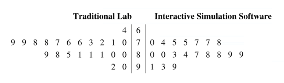
Two teaching methods and their effects on science test scores are being reviewed. A group of students is taught in traditional lab sessions. A second group of students is taught using interactive simulation software. The science test scores for the two groups are shown in the back-to-back stem-and-leaf plot.
At , α=0.01 can you support the claim that the mean science test score is lower for students taught using the traditional lab method than it is for students taught using the interactive simulation software? Assume the population variances are equal.

검증된 단계별 안내

Step 1: Formulate the null and alternative hypotheses. The null hypothesis (H₀) states that the mean science test score for students taught using the traditional lab method is equal to or greater than the mean score for students taught using interactive simulation software. The alternative hypothesis (H₁) states that the mean score for students taught using the traditional lab method is lower than the mean score for students taught using interactive simulation software.

Step 2: Extract the data from the stem-and-leaf plot. For the traditional lab method, the scores are: 99, 98, 88, 87, 76, 66, 63, 21, 10, 9, 8, 5, 11, 11, 10, 0, 0, 20, 9. For the interactive simulation software, the scores are: 46, 45, 57, 77, 78, 80, 30, 34, 47, 78, 88, 89, 99, 13, 39.

Step 3: Calculate the sample means and standard deviations for both groups. Use the formula for the sample mean:

x = \frac{\sum x}{n}

, and the formula for the sample standard deviation:

s = \sqrt{\frac{\sum (x - x) 2}{n - 1}}

. Perform these calculations for both groups.

Step 4: Conduct a two-sample t-test assuming equal variances. Use the formula for the t-statistic:

t = \frac{(x ₁ - x ₂)}{\sqrt{(s ² / n ₁) + (s ² / n ₂)}}

, where

s ²

is the pooled variance. Calculate the degrees of freedom using the formula:

df = n ₁ + n ₂ - 2

Step 5: Compare the calculated t-statistic to the critical t-value at α=0.01 for the given degrees of freedom. If the t-statistic is less than the critical t-value, reject the null hypothesis and conclude that the mean science test score is lower for students taught using the traditional lab method. Otherwise, fail to reject the null hypothesis.

비슷한 문제에 대한 검증된 영상 답변:

이 영상 해법은 위 문제에 도움이 된다고 튜터들이 추천한 것입니다.

영상 길이:

도움이 되었나요?

주요 개념

질문에 올바르게 답하기 위해 반드시 이해해야 하는 핵심 개념들은 다음과 같습니다.

Hypothesis Testing

Hypothesis testing is a statistical method used to make decisions about a population based on sample data. In this context, the null hypothesis (H0) posits that there is no difference in mean test scores between the two teaching methods, while the alternative hypothesis (H1) suggests that the mean score for the traditional lab method is lower. The significance level (α) indicates the threshold for rejecting the null hypothesis, with a common choice being 0.01 in this case.

T-test for Independent Samples

A t-test for independent samples is used to compare the means of two groups when the population variances are assumed to be equal. This test calculates a t-statistic based on the difference between the sample means, the pooled standard deviation, and the sample sizes. The resulting t-value is then compared to a critical value from the t-distribution to determine if the difference is statistically significant at the chosen alpha level.

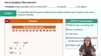
Stem-and-Leaf Plot

A stem-and-leaf plot is a graphical representation of quantitative data that helps visualize the distribution of scores. Each number is split into a 'stem' (the leading digit) and a 'leaf' (the trailing digit), allowing for easy identification of the shape and spread of the data. In this question, the stem-and-leaf plot compares the science test scores of students taught by traditional methods versus those using interactive simulations, providing a clear view of their performance.

관련 실천

교과서 질문

Constructing Confidence Intervals for μ1-μ2. You can construct a confidence interval for the difference between two population means μ1-μ2 , as shown below, when both population standard deviations are known, and either both populations are normally distributed or both n1>= 30 and n2>=30 . Also, the samples must be randomly selected and independent.

[Image]

In Exercises 29 and 30, construct the indicated confidence interval for μ1-μ2 .

Software Engineer Salaries Construct a 95% confidence interval for the difference between the mean annual salaries of entry level software engineers in Santa Clara, California, and Greenwich, CT, using the data from Exercise 27.

113

views

교과서 질문

What conditions are necessary to use the dependent samples t-test for the mean of the differences for a population of paired data?

140

views

교과서 질문

Young Adults In a survey of 3500 males ages 20 to 24 whose highest level of education is some college, but no bachelor’s degree, 80.2% were employed. In a survey of 2000 males ages 20 to 24 whose highest level of education is a bachelor’s degree or higher, 86.4% were employed. At α=0.01, can you support the claim that there is a difference in the proportion of those employed between the two groups? (Adapted from National Center for Education Statistics)

views

교과서 질문

Explain how to perform a two-sample z-test for the difference between two population means using independent samples with and known.

239

views

교과서 질문

"Testing the Difference Between Two Means In Exercises 15–24, (a) identify the claim and state Ho and Ha, (b) find the critical value(s) and identify the rejection region(s), (c) find the standardized test statistic z, (d) decide whether to reject or fail to reject the null hypothesis, and (e) interpret the decision in the context of the original claim. Assume the samples are random and independent, and the populations are normally distributed.

[APPLET] Precipitation A climatologist claims that the precipitation in Seattle, Washington, was greater than in Birmingham, Alabama, in a recent year. The daily precipitation amounts (in inches) for 30 days in a recent year in Seattle are shown below. Assume the population standard deviation is 0.25 inch.

0.00 0.00 0.05 0.01 0.21 0.00 0.00 0.52 0.00 0.010.00 0.19 0.00 0.18 0.02 0.02 0.13 0.00 0.03 0.000.04 0.00 0.41 0.23 0.00 0.80 0.15 0.00 0.00 0.79

The daily precipitation amounts (in inches) for 30 days in a recent year in Birmingham are shown below. Assume the population standard deviation is 0.52 inch.

0.00 0.96 0.84 0.00 0.10 0.00 0.00 0.20 0.00 0.54 0.97 0.00 0.35 0.02 0.04 0.70 0.00 0.00 0.00 0.00 0.03 0.01 0.15 0.27 0.00 0.00 0.93 0.00 0.89 0.01

At α=0.05, can you support the climatologist’s claim? (Source: NOAA)"

views

교과서 질문

Annual Income

A politician claims that the mean household income in a recent year is greater in York County, South Carolina, than it is in Elmore County, Alabama. In York County, a sample of 23 residents has a mean household income of \$64,900 and a standard deviation of \$16,000. In Elmore County, a sample of 19 residents has a mean household income of \$59,500 and a standard deviation of \$23,600. At , α= 0.05can you support the politician’s claim? Assume the population variances are not equal. (Adapted from U.S. Census Bureau)

views