Ch. 9 - Correlation and Regression
Larson - Elementary Statistics: Picturing the World 8th Edition
Larson8th EditionElementary Statistics: Picturing the WorldISBN: 9780137493470당신이 사용하는 게 아니라요?교과서 변경
9장, 문제 9.R.18

"In Exercises 17 and 18, use the data to (a) find the coefficient of determination r^2 and interpret
the result, and (b) find the standard error of estimate s_e and interpret the result.


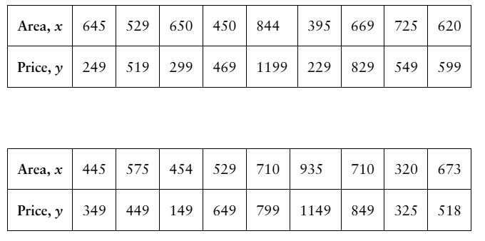
18. [APPLET] The table shows the cooking areas (in square inches) of 18 gas grills and their prices (in dollars). The regression equation is y = 1.501x - 341.501. (Source: Lowe's)

검증된 단계별 안내
1
Step 1: Calculate the coefficient of determination (r²). This involves first finding the correlation coefficient (r) between the cooking area (x) and the price (y). You can use the formula for r: r = \(\frac{n\sum xy - \sum x \sum y}{\sqrt{(n\sum x^2 - (\sum x)^2)(n\sum y^2 - (\sum y)^2)}\)}, where n is the number of data points. Then square the correlation coefficient to get r².
Step 2: Interpret the coefficient of determination (r²). Explain that r² represents the proportion of the variance in the dependent variable (price) that is predictable from the independent variable (cooking area). For example, an r² of 0.8 means 80% of the variation in price is explained by the cooking area.
Step 3: Calculate the standard error of estimate (s_e). Use the regression equation \(\hat{y}\) = 1.501x - 341.501 to find predicted prices for each cooking area. Then compute the residuals (differences between observed and predicted prices). The formula for s_e is s_e = \(\sqrt{\frac{\sum (y - \hat{y}\))^2}{n - 2}}, where n is the number of data points.
Step 4: Interpret the standard error of estimate (s_e). Explain that s_e measures the typical distance that the observed prices fall from the regression line. A smaller s_e indicates that the regression line fits the data points more closely.
Step 5: Summarize the findings by relating both r² and s_e to the quality of the regression model in predicting grill prices based on cooking area.

비슷한 문제에 대한 검증된 영상 답변:

이 영상 해법은 위 문제에 도움이 된다고 튜터들이 추천한 것입니다.
영상 길이:
1m
도움이 되었나요?

주요 개념

질문에 올바르게 답하기 위해 반드시 이해해야 하는 핵심 개념들은 다음과 같습니다.

Coefficient of Determination (r²)

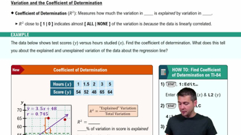
The coefficient of determination, r², measures the proportion of the variance in the dependent variable (price) that is predictable from the independent variable (area). It ranges from 0 to 1, where a higher value indicates a better fit of the regression model to the data. For example, an r² of 0.85 means 85% of the variation in price is explained by the cooking area.
추천 영상:
가이드 코스
06:14
Coefficient of Determination

Standard Error of Estimate (sₑ)

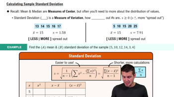
The standard error of estimate quantifies the average distance that the observed values fall from the regression line. It measures the accuracy of predictions made by the regression equation, with smaller values indicating more precise predictions. It is calculated using the residuals, which are the differences between observed and predicted values.
추천 영상:
가이드 코스
08:45
Calculating Standard Deviation

Linear Regression Equation

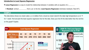
A linear regression equation models the relationship between an independent variable (area) and a dependent variable (price) using a straight line, expressed as y = mx + b. Here, y is the predicted price, x is the cooking area, m is the slope indicating the price change per unit area, and b is the y-intercept. This equation helps predict prices based on grill area.
추천 영상:
가이드 코스
07:01
Intro to Least Squares Regression
관련 실천
교과서 질문

In Exercise 26, add data for an international soccer player who can perform the half squat with a maximum of 210 kilograms and can sprint 10 meters in 2.00 seconds. Describe how this affects the correlation coefficient r.

48
views
교과서 질문

"9. Stock Price The equation used to predict the stock price (in dollars) at the end of the year for a restaurant chain is y=- 86+7.46x_1 - 1.61x_2

where x_1 is the total revenue (in billions of dollars) and x_2 is the shareholders' equity (in

billions of dollars). Use the multiple regression equation to predict the y-values for the

values of the independent variables.

a. x_1 = 27.6, x_2 = 15.3

b. x_1 = 24.1, x_2 = 14.6

c. x_1 = 23.5, x_2 = 13.4

d. x_1 = 22.8, x_2 =15.3"

57
views
교과서 질문

"[APPLET] For Exercises 1–8, use the data in the table, which shows the average annual salaries (both in thousands of dollars) for secondary and elementary school teachers, excluding special and vocational education teachers, in the United States for 11 years. (Source: U.S. Bureau of Labor Statistics)

8. Construct a 95% prediction interval for the average annual salary of elementary school teachers when the average annual salary of secondary school teachers is \$63,500. Interpret the results."

87
views
교과서 질문

"In Exercises 19-24, construct the indicated prediction interval and interpret the results.

20. Construct a 90% prediction interval for the average time adults ages 35 to 44 spend per day watching television in Exercise 10 when the average time adults ages 25 to 34 spend per day watching television is 2.25 hours."

65
views
교과서 질문

"In Exercises 19-24, construct the indicated prediction interval and interpret the results.

24. Construct a 99% prediction interval for the price of a gas grill in Exercise 18 with a usable cooking area of 900 square inches."

36
views
교과서 질문

"In Exercises 19-24, construct the indicated prediction interval and interpret the results.

23. Construct a 99% prediction interval for the top speed of an electric car in Exercise 17 that takes 5.9 seconds to accelerate from 0 to 60 miles per hour."

61
views