Ch. 3 - Describing, Exploring, and Comparing Data
Triola - Elementary Statistics 14th Edition
Triola14th EditionElementary StatisticsISBN: 9780137366446당신이 사용하는 게 아니라요?교과서 변경
3장, 문제 3.1.8

Critical Thinking. For Exercises 5–20, watch out for these little buggers. Each of these exercises involves some feature that is somewhat tricky. Find the (a) mean, (b) median, (c) mode, (d) midrange, and then answer the given question.


Geography Majors The data listed below are estimated incomes (dollars) of students who graduated from the University of North Carolina (UNC) after majoring in geography. The data are based on graduates in the year 1984. The income of basketball superstar Michael Jordan (a 1984 UNC graduate and geography major) is included. Does his income have much of an effect on the measures of center? Based on these data, would the college have been justified by saying that the mean income of a graduate in their geography program is greater than \$250,000?


17,466 18,085 17,875 19,339 19,682 19,610 18,259 16,354 2,200,000

검증된 단계별 안내
1
Step 1: Calculate the mean. The mean is the sum of all data values divided by the number of data values. Add all the incomes together, including Michael Jordan's income, and divide by the total number of data points (9 in this case). Use the formula: Mean=xn, where x is the sum of all incomes and n is the number of data points.
Step 2: Find the median. To find the median, first arrange the data in ascending order. The median is the middle value if the number of data points is odd, or the average of the two middle values if the number of data points is even. In this case, arrange the incomes and identify the middle value.
Step 3: Determine the mode. The mode is the value that appears most frequently in the dataset. Check if any income value is repeated, and if so, that value is the mode. If no value is repeated, the dataset has no mode.
Step 4: Calculate the midrange. The midrange is the average of the minimum and maximum values in the dataset. Use the formula: Midrange=Min+Max2, where Min is the smallest income and Max is the largest income.
Step 5: Analyze the effect of Michael Jordan's income. Compare the mean, median, and midrange to assess how much Michael Jordan's income skews the measures of center. Consider whether the mean is significantly higher than the median and midrange, which would indicate that his income has a large effect. Then, evaluate whether the mean income justifies the claim that the average income is greater than \$250,000.

비슷한 문제에 대한 검증된 영상 답변:

이 영상 해법은 위 문제에 도움이 된다고 튜터들이 추천한 것입니다.
영상 길이:
4m
도움이 되었나요?

주요 개념

질문에 올바르게 답하기 위해 반드시 이해해야 하는 핵심 개념들은 다음과 같습니다.

Measures of Central Tendency

Measures of central tendency, including mean, median, and mode, summarize a set of data by identifying the center point. The mean is the average of all values, the median is the middle value when data is ordered, and the mode is the most frequently occurring value. Understanding these measures is crucial for analyzing how data points, such as incomes, cluster around a central value.
추천 영상:
가이드 코스
04:52
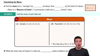
Calculating the Mean

Outliers

Outliers are data points that significantly differ from other observations in a dataset. In this context, Michael Jordan's income of $2,200,000 is an outlier that can skew the mean, making it much higher than the incomes of other geography graduates. Recognizing outliers is essential for accurately interpreting statistical measures and understanding their impact on data analysis.
추천 영상:
가이드 코스
04:48
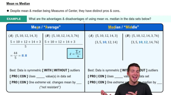
Comparing Mean vs. Median

Justification of Claims

Justifying claims about data, such as whether the mean income exceeds $250,000, requires careful analysis of the calculated measures of central tendency. This involves comparing the computed mean against the claim and considering the influence of outliers. A thorough justification ensures that conclusions drawn from the data are valid and supported by statistical evidence.
추천 영상:
가이드 코스
01:35
Step 1: Write Hypotheses Example 1
관련 실천
교과서 질문

Comparing Values. In Exercises 13–16, use z scores to compare the given values.


Tallest and Shortest Men The tallest adult male was Robert Wadlow, and his height was 272 cm. The shortest adult male was Chandra Bahadur Dangi, and his height was 54.6 cm. Heights of men have a mean of 174.12 cm and a standard deviation of 7.10 cm. Which of these two men has the height that is more extreme?

293
views
교과서 질문

Percentiles. In Exercises 17–20, use the following radiation levels (in W/kg) for 50 different cell phones. Find the percentile corresponding to the given radiation level.


1.47 W/kg

144
views
교과서 질문

Boxplots from Large Data Sets in Appendix B. In Exercises 33–36, use the given data sets in Appendix B. Use the boxplots to compare the two data sets.


Pulse Rates Use the same scale to construct boxplots for the pulse rates of males and females from Data Set 1 “Body Data” in Appendix B.

173
views
교과서 질문

Identifying Significant Values with the Range Rule of Thumb. In Exercises 33–36, use the range rule of thumb to identify the limits separating values that are significantly low or significantly high.


Foot Lengths Based on Data Set 9 “Foot and Height” in Appendix B, adult males have foot lengths with a mean of 27.32 cm and a standard deviation of 1.29 cm. Is the adult male foot length of 30 cm significantly low, significantly high, or neither? Explain.

교과서 질문

Resistant Measures Listed below are 10 wait times (minutes) for “Rock ‘n’ Roller Coaster” at 10 AM (from Data Set 33 “Disney World Wait Times”). The data are listed in order from lowest to highest. Find the mean and median of these ten values. Then find the mean and median after excluding the value of 180, which appears to be an outlier. Compare the two sets of results. How much was the mean affected by the inclusion of the outlier? How much is the median affected by the inclusion of the outlier?


15 20 25 30 30 35 45 50 50 180 

170
views
교과서 질문

In Exercises 29–32, compute the mean of the data summarized in the frequency distribution. Also, compare the computed means to the actual means obtained by using the original list of data values, which are as follows: (29) 31.4 minutes; (Exercise 30) 140.6 minutes; (Exercise 31) 55.2 years; (Exercise 32) 240.2 seconds.


296
views