Ch. 6 - Normal Probability Distributions
Triola - Elementary Statistics 14th Edition
Triola14th EditionElementary StatisticsISBN: 9780137366446당신이 사용하는 게 아니라요?교과서 변경
6장, 문제 6.2.38

Outliers For the purposes of constructing modified boxplots as described in Section 3-3, outliers are defined as data values that are above Q3 by an amount greater than 1.5 x IQR or below Q1 by an amount greater than 1.5 x IQR, where IQR is the interquartile range. Using this definition of outliers, find the probability that when a value is randomly selected from a normal distribution, it is an outlier.

검증된 단계별 안내
1
Step 1: Recall the definition of an outlier. An outlier is a data value that is either greater than Q3 + 1.5 × IQR or less than Q1 - 1.5 × IQR, where Q1 and Q3 are the first and third quartiles, respectively, and IQR (interquartile range) is defined as Q3 - Q1.
Step 2: For a normal distribution, the quartiles Q1 and Q3 correspond to specific z-scores. Q1 corresponds to the 25th percentile, and Q3 corresponds to the 75th percentile. Using a z-score table or standard normal distribution properties, these z-scores are approximately -0.674 and 0.674, respectively.
Step 3: Calculate the IQR in terms of z-scores. Since IQR = Q3 - Q1, substitute the z-scores: IQR = 0.674 - (-0.674) = 1.348.
Step 4: Determine the z-score boundaries for outliers. The boundaries are Q3 + 1.5 × IQR and Q1 - 1.5 × IQR. Substituting the values: Upper boundary = 0.674 + 1.5 × 1.348, and Lower boundary = -0.674 - 1.5 × 1.348.
Step 5: Use the standard normal distribution to find the probability of being outside these boundaries. This involves calculating the cumulative probability for the lower boundary and subtracting it from 1 minus the cumulative probability for the upper boundary. Use a z-score table or statistical software to find these probabilities.

비슷한 문제에 대한 검증된 영상 답변:

이 영상 해법은 위 문제에 도움이 된다고 튜터들이 추천한 것입니다.
영상 길이:
6m
도움이 되었나요?

주요 개념

질문에 올바르게 답하기 위해 반드시 이해해야 하는 핵심 개념들은 다음과 같습니다.

Outliers

Outliers are data points that significantly differ from other observations in a dataset. In the context of boxplots, they are defined as values that lie beyond the thresholds set by the first quartile (Q1) and the third quartile (Q3), specifically those that are more than 1.5 times the interquartile range (IQR) above Q3 or below Q1. Identifying outliers is crucial for understanding data distribution and ensuring accurate statistical analysis.
추천 영상:
가이드 코스
04:48
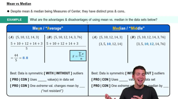
Comparing Mean vs. Median

Interquartile Range (IQR)

The interquartile range (IQR) is a measure of statistical dispersion that represents the range within which the central 50% of data points lie. It is calculated as the difference between the third quartile (Q3) and the first quartile (Q1). The IQR is particularly useful for identifying outliers, as it provides a robust measure of variability that is less affected by extreme values compared to the overall range.
추천 영상:
가이드 코스
05:45
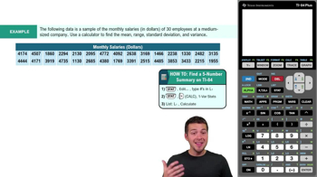
Find 5-Number Summary - TI-84 Calculator Example 1

Normal Distribution

A normal distribution is a continuous probability distribution characterized by its bell-shaped curve, where most observations cluster around the mean, and probabilities for values further away from the mean taper off symmetrically. In a normal distribution, approximately 68% of values fall within one standard deviation of the mean, and about 95% fall within two standard deviations. Understanding the properties of normal distribution is essential for calculating probabilities related to outliers.
추천 영상:
가이드 코스
09:47
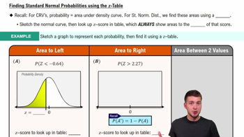
Finding Standard Normal Probabilities using z-Table
관련 실천
교과서 질문

Standard Normal Distribution. In Exercises 13–16, find the indicated z score. The graph depicts the standard normal distribution of bone density scores with mean 0 and standard deviation 1.


265
views
교과서 질문

Car Colors

In Exercises 9–12, assume that 100 cars are randomly selected. Refer to the accompanying graph, which shows the top car colors and the percentages of cars with those colors (based on PPG Industries).


Black Cars Find the probability that at least 25 cars are black. Is 25 a significantly high number of black cars?

125
views
교과서 질문

Determining Normality. In Exercises 9–12, refer to the indicated sample data and determine whether they appear to be from a population with a normal distribution. Assume that this requirement is loose in the sense that the population distribution need not be exactly normal, but it must be a distribution that is roughly bell-shaped.


Taxi Trips The distances (miles) traveled by New York City taxis transporting customers, as listed in Data Set 32 “Taxis” in Appendix B

163
views
교과서 질문

Basis for the Range Rule of Thumb and the Empirical Rule. In Exercises 45–48, find the indicated area under the curve of the standard normal distribution; then convert it to a percentage and fill in the blank. The results form the basis for the range rule of thumb and the empirical rule introduced in Section 3-2.


About __ % of the area is between z = -3.5 and z = 3.5 (or within 3.5 standard deviation of the mean).

184
views
교과서 질문

Constructing Normal Quantile Plots. In Exercises 17–20, use the given data values to identify the corresponding z scores that are used for a normal quantile plot, then identify the coordinates of each point in the normal quantile plot. Construct the normal quantile plot, then determine whether the data appear to be from a population with a normal distribution.


Earthquake Depths A sample of depths (km) of earthquakes is obtained from Data Set 24 “Earthquakes” in Appendix B: 17.3, 7.0, 7.0, 7.0, 8.1, 6.8.

139
views
교과서 질문

Finding Bone Density Scores. In Exercises 37–40 assume that a randomly selected subject is given a bone density test. Bone density test scores are normally distributed with a mean of 0 and a standard deviation of 1. In each case, draw a graph, then find the bone density test score corresponding to the given information. Round results to two decimal places.


Find P99, the 99th percentile. This is the bone density score separating the bottom 99% from the top 1%.

184
views