Business Calculus: Integration, Applications, and Multivariable Calculus

Antidifferentiation and Indefinite Integrals

Definition and Basic Concepts

Antidifferentiation is the process of finding a function whose derivative is a given function. If f(x) is a function, then a function F(x) is called an antiderivative of f(x) if F'(x) = f(x). The set of all antiderivatives of f(x) is written as an indefinite integral:

• Notation: $\int f(x)\,dx = F(x) + C$

• C is the constant of integration, representing the family of all antiderivatives.

Example: If f(x) = 2x, then F(x) = x^2 is an antiderivative, since $\frac{d}{dx}x^2 = 2x$.

Rules of Antidifferentiation

• Constant Rule: $\int k\,dx = kx + C$

• Power Rule: $\int x^n\,dx = \frac{1}{n+1}x^{n+1} + C$, for $n \neq -1$

• Natural Logarithm Rule: $\int \frac{1}{x}\,dx = \ln x + C$, for $x > 0$

• Exponential Rule: $\int e^{ax}\,dx = \frac{1}{a}e^{ax} + C$

Properties:

• A constant factor can be moved outside the integral: $\int k f(x)\,dx = k \int f(x)\,dx$

• The integral of a sum/difference is the sum/difference of the integrals: $\int [f(x) \pm g(x)]\,dx = \int f(x)\,dx \pm \int g(x)\,dx$

Initial Value Problems (IVPs)

Sometimes, an initial condition is given to solve for the constant C in the antiderivative. This is common in applied problems where a specific solution is needed.

• Step 1: Find the indefinite integral.

• Step 2: Use the initial condition to solve for C.

• Step 3: Substitute C back into the general solution.

Area and Definite Integrals

Riemann Sums and Area Approximation

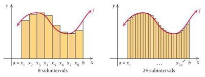
The area under a curve y = f(x) over an interval [a, b] can be approximated by dividing the interval into subintervals and summing the areas of rectangles (Riemann sums):

• Width of each rectangle: $\Delta x = \frac{b-a}{n}$

• Height: $f(x_i)$ at chosen sample points

• Approximate area: $\sum_{i=1}^n f(x_i)\Delta x$

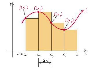
As the number of subintervals increases, the approximation becomes more accurate.

Definite Integrals and the Fundamental Theorem of Calculus

The definite integral gives the exact area under a continuous function f(x) from a to b:

• $\int_a^b f(x)\,dx = F(b) - F(a)$, where F is any antiderivative of f.

• a and b are called the limits of integration.

This is the Fundamental Theorem of Calculus, connecting differentiation and integration.

Area Above and Below the x-axis

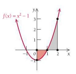
The definite integral computes the net area: area above the x-axis is positive, area below is negative.

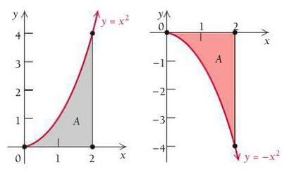
For functions that cross the x-axis, the definite integral gives the difference between the areas above and below the axis.

Applications of Definite Integrals

• Total profit from marginal profit: Integrate the marginal profit function over the relevant interval.

• Distance from velocity: Integrate the velocity function to find displacement or total distance traveled.

Integration Techniques: Substitution

Integration by Substitution

Substitution is used to simplify integrals, especially when the integrand is a composite function. It is the reverse process of the Chain Rule in differentiation.

• Let u = g(x), then du = g'(x)dx.

• Rewrite the integral in terms of u and integrate.

• Substitute back to the original variable after integrating.

This method is essential for integrating functions raised to powers or involving products of functions.

Applications: Consumer and Producer Surplus

Market Equilibrium and Surplus

The demand curve p = D(x) shows the price consumers are willing to pay for x units. The supply curve p = S(x) shows the price producers are willing to accept. The equilibrium point is where demand equals supply.

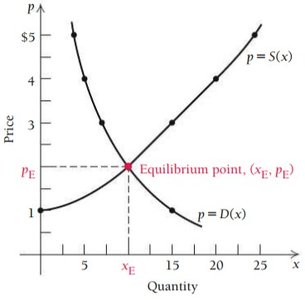
• Consumer Surplus: $\int_0^{x_E} D(x)dx - x_E p_E$

• Producer Surplus: $x_E p_E - \int_0^{x_E} S(x)dx$

These surpluses measure the benefits to consumers and producers at market equilibrium.

Applications: Accumulated Value of Continuous Income Streams

Future Value with Continuous Compounding

• Future Value: $P(t) = P_0 e^{kt}$, where P_0 is the initial investment, k is the interest rate, and t is time in years.

• Accumulated Future Value of a Continuous Income Stream: $A = e^{kT} \int_0^T R(t)e^{-kt}dt$

• If R(t) is constant: $A = \frac{R}{k}(e^{kT} - 1)$

Present Value with Continuous Compounding

• Present Value: $P_0 = P e^{-kt}$

• Accumulated Present Value of a Continuous Income Stream: $B = \int_0^T R(t)e^{-kt}dt$

• If R(t) is constant: $B = \frac{R}{k}(1 - e^{-kT})$

Functions of Several Variables: Partial Derivatives and Cobb-Douglas Production

Partial Derivatives

For a function of two variables, f(x, y), the partial derivative with respect to x is found by treating y as a constant and differentiating with respect to x:

• $\frac{\partial f}{\partial x}$ or $f_x(x, y)$

• Similarly, $\frac{\partial f}{\partial y}$ or $f_y(x, y)$

Example: For f(x, y) = x^2y^3 + xy + 4y^2:

• $\frac{\partial f}{\partial x} = 2xy^3 + y$

• $\frac{\partial f}{\partial y} = 3x^2y^2 + x + 8y$

Cobb-Douglas Production Function

The Cobb-Douglas function models production output as a function of labor and capital:

• $p(x, y) = A x^a y^{1-a}$, where $A > 0$ and $0 < a < 1$

• $\frac{\partial p}{\partial x}$: Marginal productivity of labor

• $\frac{\partial p}{\partial y}$: Marginal productivity of capital

These partial derivatives measure the rate of change of output with respect to changes in labor or capital, holding the other variable constant.