Business Calculus: Limits, Continuity, and Differentiation

Chapter 1: Differentiation

Section 1.1: Limits – A Numerical and Graphical Approach

Limits are foundational to calculus, describing the behavior of functions as inputs approach specific values. Understanding limits is essential for defining derivatives and continuity.

• Definition of Limit: The limit of f(x) as x approaches a is L if the values of f(x) get arbitrarily close to L as x gets close to a (but not equal to a).

• Notation: $\lim\limits_{x \to a} f(x) = L$

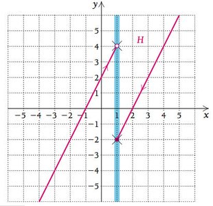
• Left-Hand and Right-Hand Limits: $\lim\limits_{x \to a^-} f(x)$ (from the left), $\lim\limits_{x \to a^+} f(x)$ (from the right). The overall limit exists only if both are equal.

• Numerical Approach: Evaluate the function at values increasingly close to a from both sides.

• Graphical Approach: Observe the behavior of the graph as x approaches a.

Example: For the sequence 2.24, 2.249, 2.2499, ..., the limit is 2.25 as x approaches 2.25 from the left.

Theorem: If both left and right limits exist and are equal, the limit exists and equals that value.

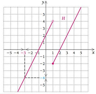
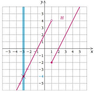
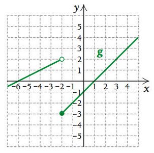
Piecewise Functions and Limits

Piecewise functions may have different behaviors on different intervals, affecting the existence of limits at certain points.

• If the left and right limits at a point are not equal, the limit does not exist at that point.

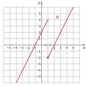
Graphical and Tabular Analysis

Tables and graphs are useful for estimating limits, especially for piecewise or discontinuous functions.

The "Wall" Method

This visual method involves drawing a vertical line ("wall") at the point of interest and observing the approach from both sides. If the function approaches the same value from both sides, the limit exists.

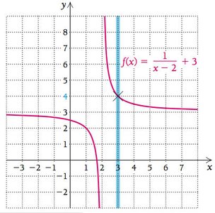
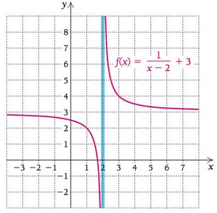
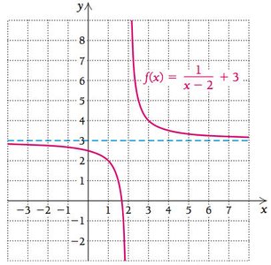
Limits Involving Rational Functions

For rational functions, direct substitution is valid if the denominator is nonzero at the point. If substitution yields an indeterminate form (0/0), algebraic simplification is required.

Summary of Limits

• The limit may exist even if the function is undefined at that point.

• Left and right limits must agree for the limit to exist.

• Graphical and numerical methods are essential tools for evaluating limits.

Section 1.2: Algebraic Limits and Continuity

Algebraic properties of limits allow for efficient calculation and analysis of function behavior. Continuity is a key property for differentiability.

• Limit Properties:

  • L1: $\lim\limits_{x \to a} c = c$

  • L2: $\lim\limits_{x \to a} [f(x)]^n = [\lim\limits_{x \to a} f(x)]^n$

  • L3: $\lim\limits_{x \to a} [f(x) \pm g(x)] = \lim\limits_{x \to a} f(x) \pm \lim\limits_{x \to a} g(x)$

  • L4: $\lim\limits_{x \to a} [f(x)g(x)] = \lim\limits_{x \to a} f(x) \cdot \lim\limits_{x \to a} g(x)$

  • L5: $\lim\limits_{x \to a} \frac{f(x)}{g(x)} = \frac{\lim\limits_{x \to a} f(x)}{\lim\limits_{x \to a} g(x)}$, if denominator ≠ 0

  • L6: $\lim\limits_{x \to a} [c f(x)] = c \cdot \lim\limits_{x \to a} f(x)$

• Continuity at a Point: A function f is continuous at x = a if:

  1. f(a) exists

  2. $\lim\limits_{x \to a} f(x)$ exists

  3. $\lim\limits_{x \to a} f(x) = f(a)$

Example: For $f(x) = \frac{x^2 - 9}{x - 3}$, direct substitution at $x=3$ gives 0/0, but factoring and simplifying yields the limit.

Section 1.3: Average Rates of Change

The average rate of change measures how a function's output changes per unit change in input over an interval. This concept is foundational for understanding derivatives.

• Formula: $\frac{f(x_2) - f(x_1)}{x_2 - x_1}$

• Difference Quotient: $\frac{f(x+h) - f(x)}{h}$, where $h \neq 0$

• Secant Line: The line connecting two points on the graph of a function; its slope is the average rate of change.

Example: For $f(x) = x^2$, the average rate of change from $x=1$ to $x=3$ is $\frac{9-1}{3-1} = 4$.

Section 1.4: Differentiation Using Limits of Difference Quotients

The derivative measures the instantaneous rate of change of a function, defined as the limit of the difference quotient as the interval approaches zero.

• Definition: $f'(x) = \lim\limits_{h \to 0} \frac{f(x+h) - f(x)}{h}$

• Geometric Interpretation: The derivative at a point is the slope of the tangent line to the curve at that point.

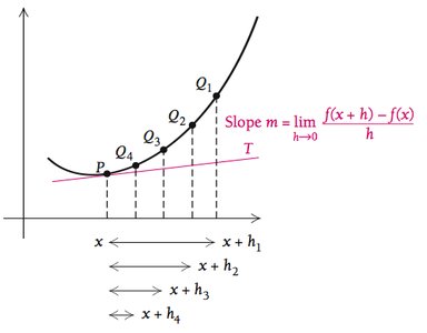
Example: For $f(x) = x^2$, $f'(x) = 2x$.

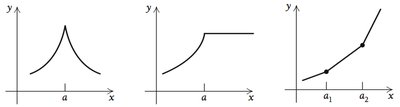
Where a Function is Not Differentiable

• At a corner or cusp

• At a point of discontinuity

• At a vertical tangent

Section 1.5: Leibniz Notation and the Power and Sum-Difference Rules

Leibniz notation and differentiation rules streamline the process of finding derivatives for common functions.

• Leibniz Notation: $\frac{dy}{dx}$ denotes the derivative of $y$ with respect to $x$.

• Power Rule: $\frac{d}{dx} x^k = kx^{k-1}$ for any real number $k$.

• Constant Rule: The derivative of a constant is zero: $\frac{d}{dx} c = 0$.

• Constant Multiple Rule: $\frac{d}{dx} [c f(x)] = c f'(x)$

• Sum-Difference Rule: $\frac{d}{dx} [f(x) \pm g(x)] = f'(x) \pm g'(x)$

Example: $\frac{d}{dx} (3x^2 + 5x - 7) = 6x + 5$

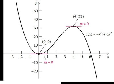
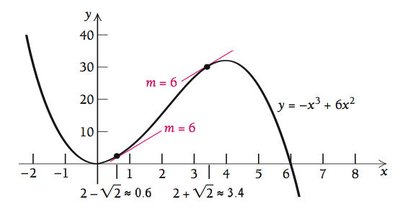
Finding Tangent Lines with Specified Slopes

To find where the tangent line to a curve has a given slope, set the derivative equal to that slope and solve for $x$.

Summary Table: Differentiation Rules

Rule	Formula
Power Rule	$\frac{d}{dx} x^k = kx^{k-1}$
Constant Rule	$\frac{d}{dx} c = 0$
Constant Multiple	$\frac{d}{dx} [c f(x)] = c f'(x)$
Sum/Difference	$\frac{d}{dx} [f(x) \pm g(x)] = f'(x) \pm g'(x)$

Key Takeaways

• Limits describe function behavior near points and are essential for defining derivatives and continuity.

• Continuity requires the function value and the limit to agree at a point.

• The derivative is the limit of the average rate of change as the interval shrinks to zero.

• Differentiation rules (power, sum, constant) simplify finding derivatives for polynomials and other functions.

• Not all continuous functions are differentiable; corners, cusps, and discontinuities prevent differentiability.