Business Calculus Study Notes: Further Optimization Problems (Inventory Control & Area Maximization)

Further Optimization Problems

Inventory Control in Business

Inventory control is a fundamental optimization problem faced by businesses that sell physical goods. The goal is to balance the costs associated with storing excess inventory (carrying costs) and the costs incurred from placing frequent orders (ordering costs).

• Carrying Costs: Expenses related to storing inventory, including space, maintenance, and refrigeration. These costs increase with larger, less frequent orders.

• Ordering Costs: Expenses incurred each time an order is placed, such as transportation fees. These costs increase with more frequent, smaller orders.

• Optimization Goal: Find the order size and frequency that minimizes the total cost (carrying + ordering).

• Average Inventory: If orders are evenly spaced and each arrives as the previous is exhausted, the average inventory is half the order size.

Example: A grocery store manager estimates annual sales of 1200 cases of frozen orange juice. Ordering cost per delivery is $75, and storage cost per case per year is $8 (applied to average inventory). The task is to determine the economic order quantity (EOQ) that minimizes total cost.

Economic Order Quantity (EOQ) Formula:

The EOQ model is used to determine the optimal order size:

$EOQ = \sqrt{\frac{2DS}{H}}$

• D: Annual demand (units/year)

• S: Ordering cost per order

• H: Carrying cost per unit per year

Application: Using the EOQ formula, the manager can calculate the optimal order size and number of orders per year to minimize costs.

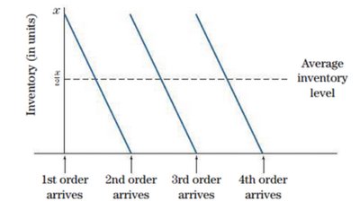
Graph Explanation: The graph illustrates inventory levels over time, with each order arriving as the previous inventory is depleted. The dashed line represents the average inventory level, which is half the order size when orders are evenly spaced.

Optimization Example: Maximizing Area with Constraints

Optimization problems often involve maximizing or minimizing a quantity subject to constraints. In this example, a farmer has a fixed amount of fencing and must determine the dimensions of two corrals (one square, one rectangular) to maximize their combined area.

• Constraint: Total fencing available is 204 meters.

• Corrals: One is square; the other is rectangular with length twice its width.

• Objective: Find the dimensions that maximize the combined area.

Method: Set up equations for perimeter and area, express all variables in terms of one variable using the constraint, and use calculus (derivatives) to find the maximum.

General Steps for Optimization:

1. Define variables and write equations for the quantity to be optimized.

2. Express the constraint as an equation.

3. Combine equations to express the objective in terms of a single variable.

4. Take the derivative and set it to zero to find critical points.

5. Check endpoints and critical points to determine the maximum or minimum.

Example: Let x be the side of the square corral, and w the width of the rectangular corral (length = 2w). The total perimeter is 4x + 6w = 204. The combined area is x2 + 2w2. Substitute and optimize using calculus.

Optimization in Business Calculus: These problems illustrate how calculus is used to solve real-world business and economic problems by finding optimal values under constraints.