Chapter 4: Graphing and Optimization – Business Calculus Study Notes

Chapter 4: Graphing and Optimization

4.1 – First Derivative & Graphs

The first derivative of a function provides essential information about the behavior of its graph, including intervals of increase, decrease, and constancy. Understanding these intervals is crucial for analyzing and sketching functions in business calculus.

• Increasing Interval: A function f is increasing on an interval (a, b) if for any x_1 < x_2 in (a, b), f(x_2) > f(x_1).

• Decreasing Interval: f is decreasing on (a, b) if f(x_2) < f(x_1) for x_1 < x_2.

• Constant Interval: f is constant if f(x_2) = f(x_1) for all x_1, x_2 in the interval.

Theorem 1 (Increasing & Decreasing Functions): For an interval (a, b):

• If f'(x) > 0, then f is increasing.

• If f'(x) < 0, then f is decreasing.

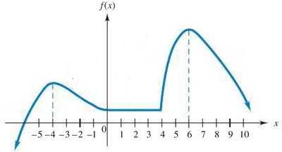
Example: The graph below can be used to identify intervals where the function is increasing, decreasing, or constant.

Critical Numbers and Local Extrema

Critical numbers are values in the domain of f where f'(x) = 0 or f'(x) does not exist. These points are candidates for local maxima or minima (collectively called local extrema).

• Local Maximum: f has a local maximum at c if f(x) ≤ f(c) for all x near c.

• Local Minimum: f has a local minimum at c if f(x) ≥ f(c) for all x near c.

First Derivative Test:

• If f' changes from positive to negative at c, f has a local maximum at c.

• If f' changes from negative to positive at c, f has a local minimum at c.

• If f' does not change sign at c, f has no local extremum at c.

4.2 – Second Derivatives & Graphs

The second derivative, f''(x), provides information about the concavity of a function and helps identify inflection points, where the concavity changes.

• Concave Up: If f''(x) > 0 on an interval, f is concave upward there.

• Concave Down: If f''(x) < 0 on an interval, f is concave downward there.

• Inflection Point: A point c where f is continuous and the concavity changes.

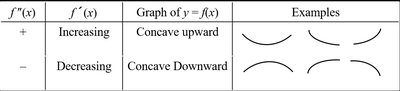
Table: Relationship Between Second Derivative, First Derivative, and Graph Shape

f''(x)	f'(x)	Graph of y = f(x)	Examples
+	Increasing	Concave upward	Upward-opening curves
-	Decreasing	Concave downward	Downward-opening curves

Second Derivative Test for Local Extrema

The second derivative test helps classify critical points as local maxima or minima:

• If f'(c) = 0 and f''(c) > 0, then f(c) is a local minimum.

• If f'(c) = 0 and f''(c) < 0, then f(c) is a local maximum.

• If f'(c) = 0 and f''(c) = 0, the test does not apply.

Table: Second Derivative Test Summary

f'(c)	f''(c)	Graph of f is:	f(c)	Example
0	+	Concave upward	Local minimum	Upward-opening curve
0	-	Concave downward	Local maximum	Downward-opening curve
0	0	?	Test does not apply	–

4.3 – L’Hospital’s Rule

L’Hospital’s Rule is a powerful tool for evaluating limits that result in indeterminate forms such as 0/0 or ∞/∞. It states that if \lim_{x \to c} f(x) = 0 and \lim_{x \to c} g(x) = 0 (or both are infinite), then:

$\lim_{x \to c} \frac{f(x)}{g(x)} = \lim_{x \to c} \frac{f'(x)}{g'(x)}$

provided the limit on the right exists or is ±∞.

• Always check that the original limit is indeterminate before applying L’Hospital’s Rule.

• Do not use the quotient rule; differentiate numerator and denominator separately.

4.5 – Absolute Maxima & Minima

Absolute extrema are the highest and lowest values a function attains on a given interval. The Extreme Value Theorem guarantees their existence for continuous functions on closed intervals.

• Absolute Maximum: f has an absolute maximum at c if f(x) ≤ f(c) for all x in the domain.

• Absolute Minimum: f has an absolute minimum at c if f(x) ≥ f(c) for all x in the domain.

Procedure for Finding Absolute Extrema:

1. Check that f is continuous on [a, b].

2. Find critical numbers in (a, b).

3. Evaluate f at endpoints and critical numbers.

4. The largest value is the absolute maximum; the smallest is the absolute minimum.

4.6 – Optimization

Optimization involves finding the maximum or minimum value of a function, often subject to constraints. This is a common application in business for maximizing profit or minimizing cost.

1. Read and understand the problem.

2. Sketch a diagram if possible.

3. Express the quantity to be optimized as a function of one variable.

4. Determine the domain.

5. Find critical numbers and evaluate endpoints if necessary.

6. Apply the appropriate test (EVT or CPT) to identify the optimum value.

Example: Maximizing the area of a fenced garden with a fixed budget, or maximizing revenue given a price-demand relationship.

Summary Table: Concavity and Extrema

Test	Condition	Conclusion
First Derivative Test	Sign change in f' at c	Local max/min at c
Second Derivative Test	f'(c) = 0, f''(c) ≠ 0	Local max if f''(c) < 0, min if f''(c) > 0
L’Hospital’s Rule	0/0 or ∞/∞ form	Take derivatives of numerator and denominator

Additional info: The included images and tables reinforce the concepts of increasing/decreasing intervals, concavity, and the application of the first and second derivative tests for extrema. The procedures and theorems summarized here are foundational for business calculus applications in graphing and optimization.