The Constant e and Continuous Compound Interest-Chapter 3

Additional Derivative Topics

The Constant e and Continuous Compound Interest

This section explores the mathematical constant e, its significance in calculus, and its application to continuous compound interest. These concepts are foundational in business calculus, especially for modeling exponential growth in finance and economics.

The Constant e

e is an irrational number approximately equal to 2.71828. It serves as the base for natural exponential and logarithmic functions, which are essential in calculus and financial mathematics.

• Definition: The number e can be defined by the following limits:

  • $e = \lim_{n \to \infty} \left(1 + \frac{1}{n}\right)^n$

  • $e = \sum_{k=0}^{\infty} \frac{1}{k!}$

• Properties:

  • e is irrational (cannot be expressed as a fraction of two integers).

  • It is the unique base for which the derivative of $e^x$ is itself: $\frac{d}{dx} e^x = e^x$.

Compound Interest

Interest can be calculated in several ways, with continuous compounding being the most mathematically significant for calculus. The formulas below describe how an investment grows over time under different compounding methods.

• Simple Interest: $A = P(1 + rt)$

• Compound Interest (m times per year): $A = P\left(1 + \frac{r}{m}\right)^{mt}$

• Continuous Compounding: $A = Pe^{rt}$

Where:

• P = principal (initial investment)

• r = annual interest rate (decimal)

• t = time in years

• m = number of compounding periods per year

• A = amount after time t

Theorem: Continuous Compound Interest Formula

If a principal P is invested at an annual rate r (in decimal form) compounded continuously, the amount A in the account after t years is:

$A = Pe^{rt}$

Examples of Compounding

• Example 1: Comparing Compounding Methods Suppose $1,000 is deposited at 5% interest per annum for 20 years. Calculate the final amount for each method:

  • Simple Interest: $A = 1000(1 + 0.05 \times 20) = 2000$

  • Compounded Annually: $A = 1000(1 + 0.05)^{20}$

  • Compounded Daily: $A = 1000\left(1 + \frac{0.05}{365}\right)^{365 \times 20}$

  • Compounded Continuously: $A = 1000e^{0.05 \times 20}$

• Example 2: Continuously Compounded Interest If $1,000 is invested at 6% interest compounded continuously for 5 years:

  • $A = 1000e^{0.06 \times 5} \approx 1349.86$

  • Interest earned: $1349.86 - 1000 = 349.86$

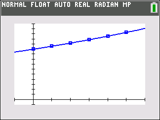
Graphing the Growth of an Investment

Continuous compounding leads to exponential growth, which can be visualized by graphing the function $A(t) = Pe^{rt}$ over time. For example, a $1,000 investment at 5.75% compounded continuously over 5 years:

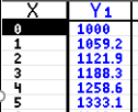
• Table of Values: The following table shows the account balance at the end of each year.

X (Years)	Y1 (Balance)
0	1000
1	1059.2
2	1121.9
3	1188.3
4	1258.6
5	1333.1

Computing Growth Time

To determine how long it takes for an investment to reach a certain value with continuous compounding, solve for t in the formula $A = Pe^{rt}$.

• Example: How long for $5,000 to grow to $8,000 at 6% compounded continuously?

  • Set $A = 8000$, $P = 5000$, $r = 0.06$

  • $8000 = 5000e^{0.06t}$

  • Divide both sides by 5000: $1.6 = e^{0.06t}$

  • Take the natural logarithm: $\ln(1.6) = 0.06t$

  • $t = \frac{\ln(1.6)}{0.06}$

Doubling Time for Continuous Compounding

The doubling time is the time required for an investment to double in value under continuous compounding. Set $A = 2P$ in the formula $A = Pe^{rt}$:

• $2P = Pe^{rt}$

• Divide both sides by $P$: $2 = e^{rt}$

• Take the natural logarithm: $\ln(2) = rt$

• Doubling time formula: $t = \frac{\ln(2)}{r}$

This formula can be generalized for tripling, quadrupling, etc., by replacing 2 with the desired multiple.