Ch. 26 Analysis of Variance (ANOVA): Comparing Several Groups in Business Statistics

Chapter 26: Analysis of Variance (ANOVA)

26.1 Comparing Several Groups

Analysis of Variance (ANOVA) is a statistical method used to compare the means of three or more groups to determine if at least one group mean is significantly different from the others. In business statistics, ANOVA is often applied using regression models with dummy variables to analyze experimental or observational data involving categorical explanatory variables.

Comparing Groups: The Wheat Variety Example

• Scenario: Five wheat varieties (Endurance, Hatcher, NuHills, RonL, Ripper) are tested for yield (bushels per acre) in a balanced experiment (equal observations per group).

• Purpose: To determine if yield differences are due to variety, temperature, or random chance.

• Steps in ANOVA:

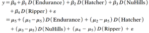
  1. Plot the data to visualize group differences.

  2. Propose a regression model with dummy variables for each group.

  3. Check model assumptions (independence, equal variances, normality).

  4. Test hypotheses and draw conclusions.

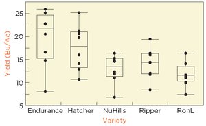
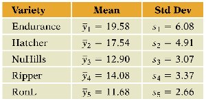
Descriptive Statistics for Each Variety

The table below summarizes the mean and standard deviation for each wheat variety:

Variety	Mean	Std Dev
Endurance	$\bar{y}_1 = 19.58$	$s_1 = 6.08$
Hatcher	$\bar{y}_2 = 17.54$	$s_2 = 4.91$
NuHills	$\bar{y}_3 = 12.90$	$s_3 = 3.07$
Ripper	$\bar{y}_4 = 14.08$	$s_4 = 3.37$
RonL	$\bar{y}_5 = 11.68$	$s_5 = 2.66$

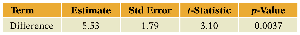
Relating the t-Test to Regression

To compare Endurance to all other varieties, a two-sample t-test can be used if variances are similar. The t-test result can be interpreted using regression with a dummy variable for Endurance:

Term	Estimate	Std Error	t-Statistic	p-Value
Difference	5.53	1.79	3.10	0.0037

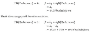
The regression model with a dummy variable for Endurance is:

• If $D(Endurance) = 0$: $\hat{y} = b_0 = 14.05$ bushels/acre (average for other varieties)

• If $D(Endurance) = 1$: $\hat{y} = b_0 + b_1 = 14.05 + 5.53 = 19.58$ bushels/acre (average for Endurance)

Regression with Multiple Dummy Variables

To compare all varieties, use J-1 dummy variables (for J groups). RonL is the baseline (all dummies = 0). The regression model is:

• $y = b_0 + b_1 D(Endurance) + b_2 D(Hatcher) + b_3 D(NuHills) + b_4 D(Ripper) + \varepsilon$

• The intercept $b_0$ is the mean for RonL; each slope $b_j$ is the difference between variety $j$ and RonL.

Term	Estimate	Std Error	t-Statistic	p-Value
Intercept	11.68	1.49	7.84	<.0001
D(Endurance)	7.90	2.11	3.75	0.0006
D(Hatcher)	5.86	2.11	2.78	0.0087
D(NuHills)	1.22	2.11	0.58	0.5682
D(Ripper)	2.40	2.11	1.14	0.2633

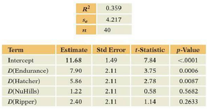
The fitted value for Hatcher is $11.68 + 5.86 = 17.54$ bushels/acre.

ANOVA Regression Model in Population Terms

The ANOVA regression model can be written as:

• $y = \mu_5 + (\mu_1 - \mu_5) D(Endurance) + (\mu_2 - \mu_5) D(Hatcher) + (\mu_3 - \mu_5) D(NuHills) + (\mu_4 - \mu_5) D(Ripper) + \varepsilon$

One-Way ANOVA Model and Assumptions

One-way ANOVA compares the means of groups defined by a single categorical variable. The model is:

• $y_{ij} = \mu_j + \varepsilon_{ij}$

• Assumptions: errors are independent, have equal variances, and are normally distributed.

26.2 Inference in ANOVA Regression Models

Before conducting inference, check the following conditions:

• Independence: Satisfied if data are from a randomized experiment.

• Equal variances: Check if group IQRs are within a factor of 3 to 1.

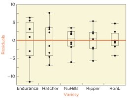
• Normality: Assess with residual plots and normal quantile plots.

F-Test for the Difference Among Means

The F-test evaluates the null hypothesis $H_0: \mu_1 = \mu_2 = \cdots = \mu_J$. The ANOVA table summarizes the test:

Source	df	Sum of Squares	Mean Square	F	p-Value
Regression	4	54.884	13.72	3.500	0.0090
Residual	35	137.322	3.923
Total	39	192.206

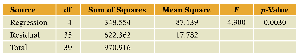
If the p-value is less than 0.05, reject $H_0$ and conclude that not all means are equal.

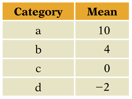
Understanding the F-Test

The F-test compares the variance between group means to the variance within groups. If between-group variance is much larger, group means are likely different. Otherwise, differences may be due to random variation.

Category	Mean
a	10
b	4
c	0
d	-2

26.3 Multiple Comparisons

When comparing multiple groups, the risk of Type I error increases. Multiple comparison procedures adjust for this risk.

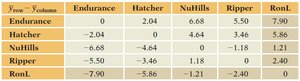
Pairwise Differences Table

	Endurance	Hatcher	NuHills	Ripper	RonL
Endurance	0	2.04	6.68	5.50	7.90
Hatcher	-2.04	0	4.64	3.46	5.86
NuHills	-6.68	-4.64	0	1.18	1.21
Ripper	-5.50	-3.46	1.18	0	2.40
RonL	-7.90	-5.86	-1.21	-2.40	0

Tukey Confidence Intervals

• Controls the overall Type I error rate at 5% for all pairwise comparisons.

• Uses a larger critical value than the t-interval, based on the number of groups.

• Example: For Endurance vs. Hatcher, the 95% Tukey interval is $2.04 \pm 6.07$ bushels/acre. Since this interval includes 0, the difference is not significant.

• Any difference must exceed 6.07 bushels/acre to be significant at the 5% level.

Bonferroni Confidence Intervals

• Adjusts the significance level for multiple comparisons: $\alpha_{adj} = \alpha / M$ for $M$ intervals.

• For 10 comparisons, $\alpha = 0.05$ becomes $0.005$; the t-critical value increases, making intervals wider and more conservative.

26.4 Groups of Different Size

When group sizes are unequal (unbalanced data), the standard errors for pairwise comparisons differ. The estimated standard error for comparing two group means is calculated using the sample sizes for each group.

Additional info: The formula for the standard error in the unbalanced case is:

$SE = s_p \sqrt{\frac{1}{n_1} + \frac{1}{n_2}}$

where $s_p$ is the pooled standard deviation, and $n_1$, $n_2$ are the sample sizes for the two groups.