Association Between Categorical Variables: Contingency Tables, Lurking Variables, and Strength of Association

Chapter 5: Association Between Categorical Variables

5.1 Contingency Tables

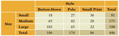
Contingency tables are a fundamental tool in business statistics for analyzing the relationship between two categorical variables. They display the frequency distribution of variables and help identify associations between them.

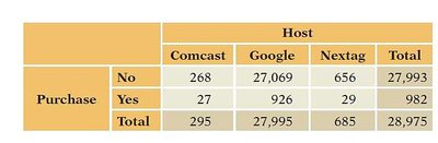
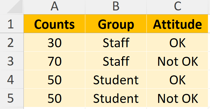
• Definition: A contingency table (also called a cross-tabulation or crosstab) shows the counts of cases for every combination of two categorical variables. Each cell represents a unique combination of the variables.

• Example: Analyzing which web hosts send more buyers to Amazon.com by cross-tabulating Host (Comcast, Google, Nextag) and Purchase (Yes/No).

Marginal and Conditional Distributions

Contingency tables allow us to compute two important types of distributions:

• Marginal Distribution: The totals for each category of a single variable, found in the margins (last row/column) of the table.

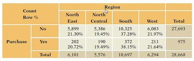
• Conditional Distribution: The distribution of one variable for a fixed value of the other variable (e.g., the percentage of purchases for each host).

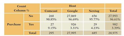
Interpretation: The conditional distribution reveals that Comcast has the highest purchase rate, indicating an association between Host and Purchase.

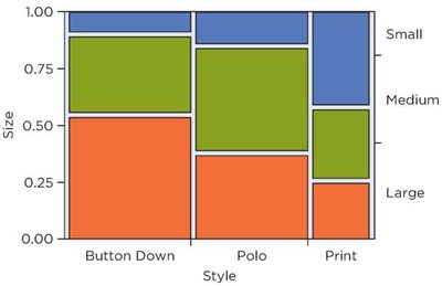
Visualizing Contingency Tables

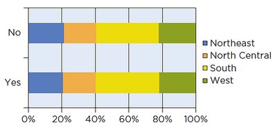
• Stacked Bar Charts: These display conditional distributions by dividing bars into segments proportional to the percentage in each group of a second variable.

• Mosaic Plots: An alternative visualization where the size of each tile is proportional to the count in a cell of the contingency table.

5.2 Lurking Variables and Simpson’s Paradox

It is important to remember that association does not imply causation. Sometimes, a third variable (a lurking variable) can influence the observed relationship between two variables, leading to misleading conclusions.

• Lurking Variable: A hidden variable that affects the apparent relationship between two other variables.

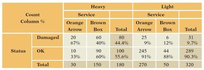
• Simpson’s Paradox: The direction or strength of an association between two variables can change when data are separated into groups defined by a third variable.

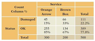
Example: Orange Arrow appears to be a better shipper until the data are separated by package weight, revealing the effect of the lurking variable.

5.3 Strength of Association

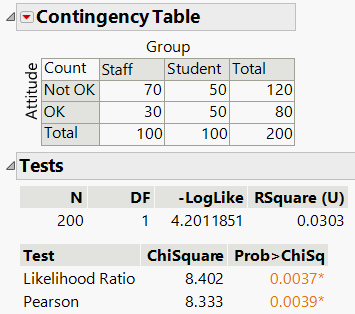
To quantify the association between categorical variables, statisticians use the Chi-Squared Statistic and related measures.

• Chi-Squared Statistic (\( \chi^2 \)): Measures how much the observed counts in a contingency table differ from the counts expected if the variables were independent.

• Formula:

$\chi^2 = \sum \frac{(\text{Observed} - \text{Expected})^2}{\text{Expected}}$

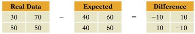
Example Calculation:

$\chi^2 = \frac{(30-40)^2}{40} + \frac{(70-60)^2}{60} + \frac{(50-40)^2}{40} + \frac{(50-60)^2}{60} = 2.5 + 1.67 + 2.5 + 1.67 = 8.33$

Cramer’s V

Cramer’s V is a normalized measure of association derived from the Chi-Squared statistic, ranging from 0 (no association) to 1 (perfect association).

• Formula:

$V = \sqrt{\frac{\chi^2}{n \times \min(r-1, c-1)}}$

• Where n is the total sample size, r is the number of rows, and c is the number of columns.

Checklist for Chi-Squared and Cramer’s V

• Verify that variables are categorical.

• Check for the presence of lurking variables before interpreting association.

Summary Table: Key Contingency Table Concepts

Concept	Definition	Example
Contingency Table	Table showing counts for combinations of two categorical variables	Host vs. Purchase
Marginal Distribution	Totals for each category of a single variable	Total Purchases by Host
Conditional Distribution	Distribution of one variable for a fixed value of another	Purchase rate for each Host
Lurking Variable	Hidden variable affecting observed association	Weight in shipping example
Simpson’s Paradox	Association changes when data are grouped by a third variable	Shipping service by weight
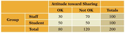
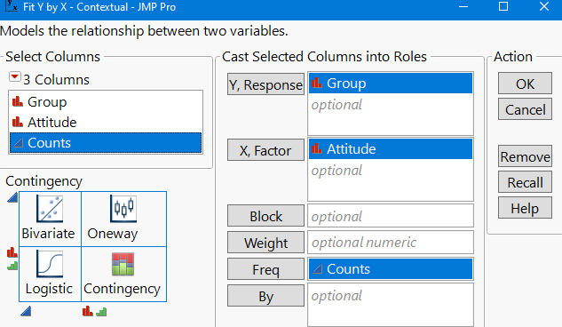
Chi-Squared Statistic	Quantifies difference between observed and expected counts	Attitude toward sharing by group
Cramer’s V	Normalized measure of association (0 to 1)	Strength of association in contingency table