Association Between Categorical Variables: Contingency Tables, Lurking Variables, and Strength of Association

Association Between Categorical Variables

Introduction

Understanding the association between categorical variables is essential in business statistics for analyzing relationships in data. This chapter explores how to summarize and interpret associations using contingency tables, visualizations, and statistical measures, while also considering the impact of lurking variables.

Contingency Tables

Definition and Purpose

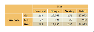
A contingency table is a tabular summary that displays the frequency distribution of variables. It is used to examine the relationship between two or more categorical variables by showing counts for each combination of categories.

• Cells in a contingency table are mutually exclusive, representing unique combinations of variable categories.

• Marginal totals (in the table's margins) show the total counts for each category of a single variable.

Marginal and Conditional Distributions

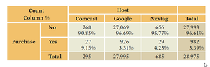
Marginal distributions are the totals for each category of a variable, found in the margins of the table. Conditional distributions show the distribution of one variable for a fixed value of another variable, often expressed as percentages within rows or columns.

• Conditional distributions help reveal associations between variables.

Interpreting Conditional Distributions

• For example, Comcast has a higher purchase rate (9.15%) compared to Google (3.31%) and Nextag (4.23%), indicating an association between host and purchase.

• If conditional distributions are similar across groups, variables are likely independent.

Visualizing Associations

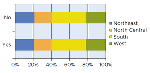
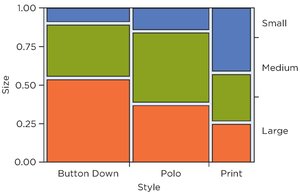
Visual tools such as stacked bar charts and mosaic plots are used to display conditional distributions and associations between categorical variables.

• Stacked bar charts divide bars into segments proportional to group percentages.

• Mosaic plots use the area of tiles to represent cell counts, visually highlighting associations.

Examples of Contingency Tables

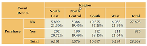
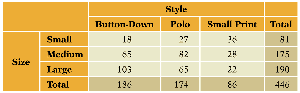
• Contingency tables can be constructed for various business scenarios, such as purchase behavior by region or shirt size by style.

Lurking Variables and Simpson’s Paradox

Lurking Variables

A lurking variable is an unobserved variable that influences the apparent relationship between two other variables. Failing to account for lurking variables can lead to misleading conclusions about associations.

Simpson’s Paradox

Simpson’s Paradox occurs when the association between two variables reverses or changes direction after accounting for a third variable. This highlights the importance of considering all relevant variables in analysis.

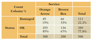
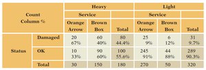
• For example, a shipping service may appear better overall, but when data are separated by package weight, the association reverses.

Strength of Association

Chi-Squared Statistic

The Chi-Squared (\( \chi^2 \)) statistic measures the strength of association between categorical variables in a contingency table. It compares observed counts to expected counts under the assumption of independence.

• Formula: $\chi^2 = \sum \frac{(O - E)^2}{E}$ where \(O\) is the observed count and \(E\) is the expected count.

• Expected counts are calculated based on marginal totals, assuming no association.

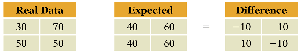
Calculating the Chi-Squared Statistic

• Sum the squared differences between observed and expected counts, divided by expected counts, across all cells.

• A large \( \chi^2 \) value suggests a strong association; a small value suggests independence.

Preparing Data for Analysis

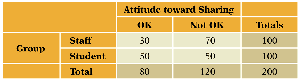
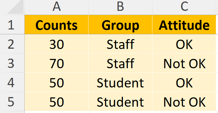
To analyze contingency tables in statistical software (e.g., JMP), data should be structured with each row representing a unique combination of variable categories and its count.

Example: JMP Output

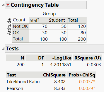
• The output provides the \( \chi^2 \) statistic and p-value, indicating whether the association is statistically significant.

Cramer’s V

Cramer’s V is a standardized measure of association derived from the chi-squared statistic. It ranges from 0 (no association) to 1 (perfect association), allowing comparison across tables of different sizes.

• Formula: $V = \sqrt{\frac{\chi^2}{n(k-1)}}$ where \(n\) is the total sample size and \(k\) is the smaller number of rows or columns.

Checklist for Chi-Squared and Cramer’s V

• Ensure variables are categorical.

• Check for lurking variables that may affect the association.

Summary Table: Key Concepts in Association Analysis

Concept	Definition	Application
Contingency Table	Tabular summary of counts for combinations of categorical variables	Examining relationships between variables
Marginal Distribution	Totals for each category of a variable	Understanding overall frequencies
Conditional Distribution	Distribution of one variable for a fixed value of another	Assessing association
Lurking Variable	Unobserved variable affecting association	Identifying confounding effects
Simpson’s Paradox	Reversal of association after accounting for a third variable	Ensuring accurate interpretation
Chi-Squared Statistic	Measure of association strength	Testing independence
Cramer’s V	Standardized measure of association	Comparing associations