Association Between Categorical Variables: Contingency Tables, Lurking Variables, and Strength of Association

Association Between Categorical Variables

Contingency Tables

Contingency tables are fundamental tools in business statistics for analyzing the relationship between two categorical variables. They display the frequency of cases for each combination of categories, allowing for the examination of possible associations.

• Definition: A contingency table shows counts of cases for each combination of two categorical variables.

• Cells: Each cell represents a unique combination and is mutually exclusive.

• Marginal Distributions: Totals for each variable, found in the table's margins.

• Conditional Distributions: Frequencies within a row or column, restricted to cases meeting a specific condition.

• Application: Used to determine if variables such as 'Host' and 'Purchase' are associated.

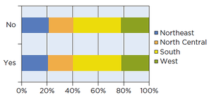
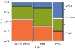
Visualizing Associations

Visual tools such as stacked bar charts and mosaic plots help illustrate associations or lack thereof between categorical variables.

• Stacked Bar Charts: Display conditional distributions by dividing bars proportionally according to group percentages.

• Mosaic Plots: Represent cell counts with tile sizes proportional to frequency, providing a visual sense of association.

Lurking Variables and Simpson’s Paradox

Lurking Variables

A lurking variable is a hidden factor that influences the apparent relationship between two other variables, potentially leading to misleading conclusions.

• Definition: A concealed variable affecting the observed association.

• Example: Shipping service appears better until adjusted for package weight.

Simpson’s Paradox

Simpson’s Paradox occurs when the association between two variables reverses or changes after accounting for a third variable.

• Definition: Change in association when data are separated by a third variable.

• Application: Important in business statistics to avoid incorrect causal interpretations.

Strength of Association

Chi-Squared Statistic

The chi-squared statistic is a measure used to assess the strength of association between categorical variables in a contingency table.

• Definition: Compares observed counts to expected counts under the assumption of no association.

• Calculation: Accumulates squared deviations between observed and expected counts across all cells.

• Formula:

$\chi^2 = \sum \frac{(O - E)^2}{E}$ Where O = observed count, E = expected count.

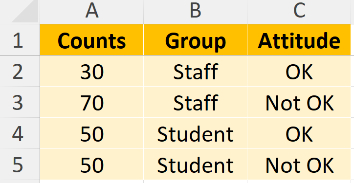
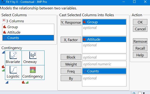
Preparing Data for Analysis

Data must be formatted correctly for statistical software analysis, such as JMP. Each count and its related information should be represented in a single row, and totals should be removed.

• Step 1: Remove total rows and columns.

• Step 2: Structure data so each row contains a count and its associated variables.

Cramer’s V

Cramer’s V is a normalized measure of association derived from the chi-squared statistic, ranging from 0 (no association) to 1 (perfect association).

• Definition: Quantifies the strength of association between categorical variables.

• Formula:

$V = \sqrt{\frac{\chi^2}{n \cdot (\min(r-1, c-1))}}$ Where $\chi^2$ is the chi-squared statistic, $n$ is the total number of observations, $r$ is the number of rows, and $c$ is the number of columns.

Checklist for Chi-Squared and Cramer’s V

• Verify that variables are categorical.

• Check for lurking variables before interpreting association.

Summary Table Examples

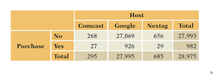
Contingency Table Example: Web Shopping

Host	Comcast	Google	Nextag	Total
No	268	27,069	656	27,993
Yes	27	926	29	982
Total	295	27,995	685	28,975

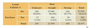
Conditional Distribution Example: Web Shopping

Host	Comcast	Google	Nextag	Total
No	268 (90.85%)	27,069 (96.66%)	656 (95.77%)	27,993 (96.61%)
Yes	27 (9.15%)	926 (3.31%)	29 (4.23%)	982 (3.39%)
Total	295	27,995	685	28,975

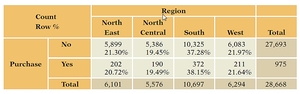
Contingency Table Example: Purchase by Region

Region	North East	North Central	South	West	Total
No	5,899 (21.30%)	5,386 (19.45%)	10,325 (37.28%)	6,083 (21.97%)	27,693
Yes	202 (20.72%)	190 (19.49%)	372 (38.15%)	211 (21.64%)	975
Total	6,101	5,576	10,697	6,294	28,668

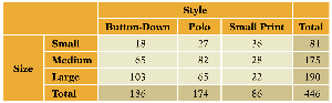
Contingency Table Example: Shirt Size by Style

Style	Button-Down	Polo	Small Print	Total
Small	19	27	35	81
Medium	65	82	28	175
Large	103	65	22	190
Total	187	174	86	447

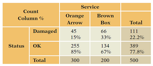
Contingency Table Example: Service Status

Service	Orange Arrow	Brown Box	Total
Damaged	45 (15%)	66 (33%)	111 (22.2%)
OK	255 (85%)	134 (67%)	389 (77.8%)
Total	300	200	500

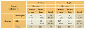
Contingency Table Example: Service Status by Weight

	Heavy			Light
Service	Orange Arrow	Brown Box	Total	Orange Arrow	Brown Box	Total
Damaged	20 (67%)	60 (40%)	80 (44.4%)	25 (9%)	6 (12%)	31 (9.7%)
OK	10 (33%)	90 (60%)	100 (55.6%)	245 (91%)	44 (88%)	289 (90.3%)
Total	30	150	180	270	50	320

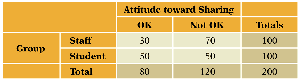
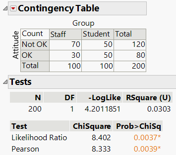
Contingency Table Example: Attitude Toward Sharing

Group	OK	Not OK	Totals
Staff	30	70	100
Student	50	50	100
Total	80	120	200

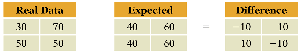
Observed vs Expected Counts Example

Real Data	Expected	Difference
30	40	10
70	60	10
50	40	10
50	80	-10

Checklist for Statistical Tests

• Ensure variables are categorical.

• Check for lurking variables before interpreting results.

Additional info: These notes expand on the original slides and tables, providing definitions, formulas, and context for business statistics students. All images included are directly relevant to the explanation of their adjacent paragraphs.