Ch 5. Association Between Categorical Variables: Contingency Tables, Lurking Variables, and Strength of Association

Chapter 5: Association Between Categorical Variables

5.1 Contingency Tables

Contingency tables are essential tools in business statistics for analyzing the relationship between two categorical variables. They display the frequency distribution of variables and help identify patterns of association.

• Definition: A contingency table (also called a cross-tabulation or two-way table) shows the counts of cases for every combination of two categorical variables. Each cell represents a mutually exclusive category.

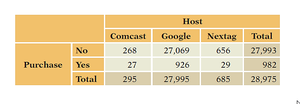
• Example: Analyzing which web hosts send more buyers to Amazon.com by cross-tabulating Host (Comcast, Google, Nextag) and Purchase (Yes/No).

Marginal and Conditional Distributions

Marginal distributions summarize the totals for each variable, while conditional distributions focus on the distribution of one variable within the levels of another.

• Marginal Distribution: The totals in the margins (bottom row and rightmost column) of the contingency table, representing the overall frequency for each category.

• Conditional Distribution: The distribution of one variable, given a specific value of the other variable (e.g., purchase rates for each host).

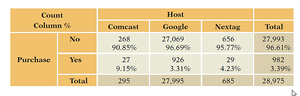
Interpretation: Comcast has the highest purchase rate (9.15%), indicating an association between Host and Purchase.

Visualizing Associations

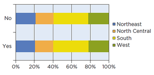
• Stacked Bar Charts: Used to display conditional distributions by dividing bars into segments proportional to group percentages.

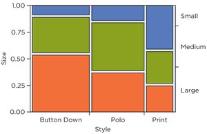
• Mosaic Plots: An alternative to stacked bar charts, where the size of each tile is proportional to the count in a cell of the contingency table.

Additional Examples

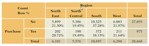
• Contingency Table of Purchase by Region: Shows the relationship between geographic region and purchase behavior.

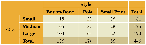
• Contingency Table of Shirt Size by Style: Illustrates the association between shirt size and style preferences.

5.2 Lurking Variables and Simpson’s Paradox

Not all observed associations imply causation. Sometimes, a hidden or lurking variable can influence the relationship between two variables, leading to misleading conclusions. Simpson’s Paradox occurs when the direction of an association reverses after accounting for a third variable.

• Lurking Variable: A variable not included in the analysis that affects the apparent relationship between the studied variables.

• Simpson’s Paradox: The phenomenon where an observed association between two variables reverses or disappears when data are separated into groups defined by a third variable.

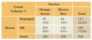
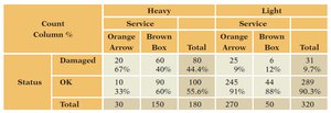
Example: Orange Arrow appears to be a better shipper until the data are separated by package weight, revealing the effect of the lurking variable.

5.3 Strength of Association

To quantify the association between categorical variables, statisticians use the Chi-Squared Statistic and derived measures such as Cramer’s V.

Chi-Squared Statistic ($\chi^2$)

• Definition: Measures the discrepancy between observed and expected counts in a contingency table, assuming no association between variables.

• Formula:

$\chi^2 = \sum_{i} \sum_{j} \frac{(O_{ij} - E_{ij})^2}{E_{ij}}$

Where $O_{ij}$ is the observed count in cell $(i, j)$ and $E_{ij}$ is the expected count under the null hypothesis of independence.

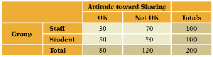
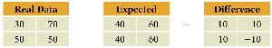
• Interpretation: A large $\chi^2$ value suggests a strong association between the variables.

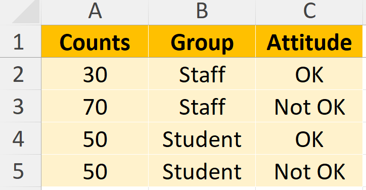
Preparing Data for Analysis

• Remove total rows and columns from the contingency table.

• Restructure the data so each row represents a unique combination of the two variables and its count.

Using JMP for Chi-Squared Test

• Open the data file in JMP.

• Use the menu: Analyze > Fit Y by X, and assign variables appropriately.

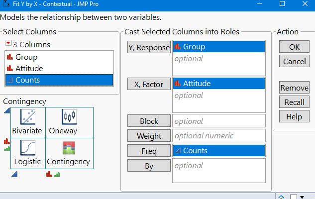
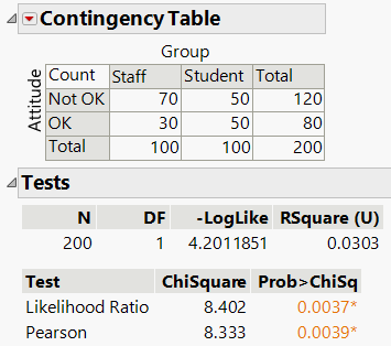
• Output: JMP provides the Chi-Squared statistic and p-value to assess the significance of the association.

Cramer’s V

• Definition: A standardized measure of association derived from the Chi-Squared statistic, ranging from 0 (no association) to 1 (perfect association).

• Formula:

$V = \sqrt{\frac{\chi^2}{n(k-1)}}$

Where $n$ is the total sample size and $k$ is the smaller number of rows or columns.

• Checklist for Validity:

  • Variables must be categorical.

  • No obvious lurking variables should be present.

Additional info: This chapter provides foundational tools for analyzing categorical data, which are essential for business decision-making, marketing analysis, and quality control. Understanding these concepts helps avoid common pitfalls such as misinterpreting associations due to lurking variables.