Ch. 24 Building Regression Models: Identifying and Evaluating Explanatory Variables

Chapter 24: Building Regression Models

24.1 Identifying Explanatory Variables

In regression analysis, selecting appropriate explanatory variables is crucial for building effective predictive models. The process often begins with theoretical guidance, such as the Capital Asset Pricing Model (CAPM) in finance, and is refined by considering additional variables that may improve model fit and predictive accuracy.

• Initial Model: The CAPM suggests using the percentage change for the whole stock market as an explanatory variable for stock returns.

• Model Building: Additional variables are considered to enhance the model, but the process is complicated by the potential for collinearity among explanatory variables.

• Example: Modeling Sony stock returns using market % change as the initial explanatory variable.

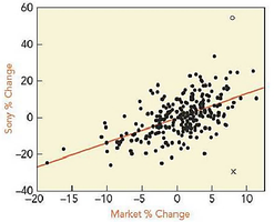
Scatterplot Analysis

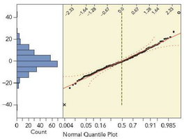
A scatterplot of Sony % Change versus Market % Change reveals a linear association, with two notable outliers.

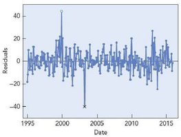
Timeplot of Residuals

Examining the residuals over time helps identify outliers and assess independence. In this case, no evidence of dependence is observed.

Regression Results

The regression output provides estimates for the intercept and slope, along with their statistical significance.

Term	Estimate	Std Error	t-stat	p-value
Intercept	-0.4610	0.5927	-0.78	0.4375
Market % Change	1.3370	0.1305	10.25	<0.0001

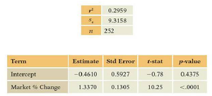
• Interpretation: The intercept is not statistically significant (p = 0.4375), while the slope for Market % Change is highly significant (p < 0.0001).

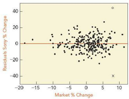
Residual Analysis

Residual plots are used to check for constant variance and normality of errors. Aside from the two outliers, residuals appear to have similar variances and are nearly normal.

Identifying Additional Variables

Research suggests adding variables such as:

• Dow % Change: Percentage change in the Dow Jones Industrial Average (DJIA)

• Small-Big: Difference in performance between small and large companies

• High-Low: Difference in performance between growth and value stocks

Correlation and Scatterplot Matrices

Correlation matrices and scatterplot matrices help assess relationships among variables and detect collinearity.

	Sony % Change	Market % Change	Dow % Change	Small-Big	High-Low
Sony % Change	1.000	0.544	0.461	0.327	-0.208
Market % Change	0.544	1.000	0.910	0.252	-0.227
Dow % Change	0.461	0.910	1.000	0.009	-0.052
Small-Big	0.327	0.252	0.009	1.000	-0.347
High-Low	-0.208	-0.227	-0.052	-0.347	1.000

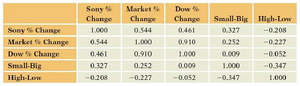
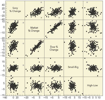
• Observation: Market % Change and Dow % Change are highly correlated (r = 0.91), indicating potential collinearity.

Multiple Regression Model (MRM)

Including all four explanatory variables in the model allows for a more comprehensive analysis. The F-statistic and t-statistics are used to assess overall and individual variable significance.

Term	Estimate	Std Error	t-stat	p-value
Intercept	-0.4340	0.5822	-0.75	0.4567
Market % Change	0.3900	0.4942	0.26	0.0525
Dow % Change	0.1913	0.4957	0.39	0.4222
Small-Big	0.5911	0.1567	3.77	0.0002
High-Low	-0.1450	0.1982	-0.73	0.4653

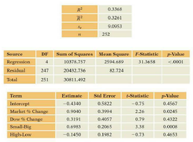
• Interpretation: The F-statistic is significant (p < 0.0001), indicating the model explains significant variation. Only Small-Big is statistically significant among the four variables.

24.2 Collinearity

Collinearity occurs when explanatory variables are highly correlated, leading to imprecise estimates of regression coefficients. This affects the interpretation and reliability of the model.

• Marginal vs. Partial Slopes: Marginal slopes are estimated without controlling for other variables, while partial slopes account for the presence of other variables. Collinearity can cause large differences between these estimates.

• Variance Inflation Factor (VIF): VIF quantifies the increase in variance of a coefficient due to collinearity. It is calculated as:

$VIF_j = \frac{1}{1 - R_j^2}$

• Where $R_j^2$ is the coefficient of determination from regressing the j-th explanatory variable on all other explanatory variables.

• VIF values greater than 5 or 10 suggest problematic collinearity.

Signs of Collinearity

• R2 increases less than expected when adding variables.

• Slopes of correlated variables change dramatically when other variables are added or removed.

• F-statistic is significant, but individual t-statistics are not.

• Standard errors for partial slopes are larger than for marginal slopes.

• Variance inflation factors increase.

Addressing Collinearity

• Remove redundant explanatory variables.

• Re-express variables (e.g., use averages or principal components).

• Retain variables if they are significant and estimates are sensible.

24.3 Removing Explanatory Variables

Not all explanatory variables in a regression model may be statistically significant. Removing non-significant variables can simplify the model without substantially reducing explanatory power (R2), provided they do not introduce collinearity. However, variables of theoretical or practical interest may be retained if justified.

• Key Principle: Remove variables that are not significant and do not contribute to the model, unless they are of special interest and do not cause collinearity.