Business Statistics: Foundational Concepts and Descriptive Measures

Defining and Collecting Data

Introduction to Business Analytics and Statistics

Business analytics involves using statistical methods and technologies to analyze historical data, gain insights, and improve decision-making. Statistics is a branch of mathematics focused on collecting, analyzing, interpreting, and presenting data. The DCOVA framework guides statistical analysis: Define, Collect, Organize, Visualize, and Analyze.

• Descriptive Statistics: Summarize and present data (e.g., mean, median, variance).

• Inferential Statistics: Draw conclusions about populations from samples (e.g., estimation, hypothesis testing).

• Predictive Statistics: Use models to forecast future outcomes.

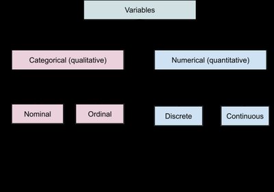
Variables and Types of Data

Variables are characteristics or attributes measured in a study. Data are the observed values of these variables. Variables can be classified as categorical (qualitative) or numerical (quantitative), with further subdivisions:

• Categorical (Qualitative): Nominal (no order), Ordinal (ordered categories)

• Numerical (Quantitative): Discrete (countable values), Continuous (any value within a range)

Levels of Measurement

The level of measurement determines the mathematical properties of data:

• Nominal: Categories without order (e.g., gender, eye color)

• Ordinal: Ordered categories (e.g., satisfaction ratings)

• Interval: Numeric, equal intervals, no true zero (e.g., temperature in Celsius)

• Ratio: Numeric, equal intervals, true zero (e.g., height, weight, revenue)

Sampling Methods

Sampling is the process of selecting a subset of a population for analysis. There are two main types:

• Non-probability Samples: Judgement, convenience, quota, self-selection (not random, may introduce bias)

• Probability Samples: Simple random, stratified, systematic, cluster (random selection, allows inference to population)

Tabular and Visual Summarization of Variables

Measures of Central Tendency

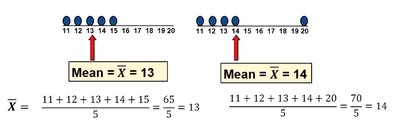
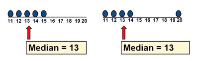
Central tendency describes the center of a data set. The three main measures are:

• Mean: Arithmetic average, sensitive to outliers.

• Median: Middle value when data are ordered, robust to outliers.

• Mode: Most frequent value, useful for categorical data.

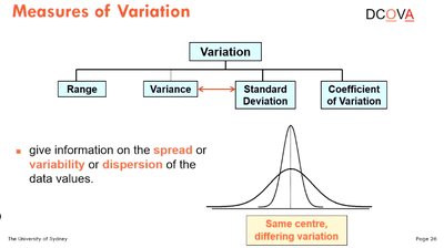
Measures of Variation

Variation measures the spread or dispersion of data values. Key measures include:

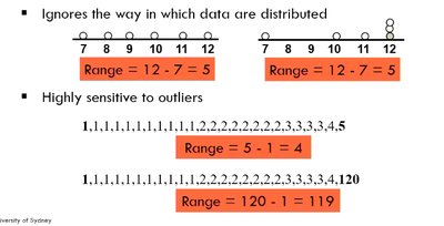
• Range: Difference between largest and smallest values. Sensitive to outliers.

• Variance: Average squared deviation from the mean.

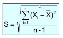
• Standard Deviation: Square root of variance, in same units as data.

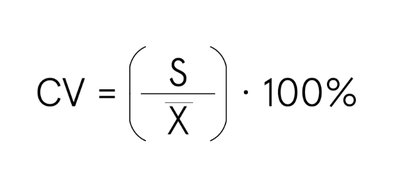
• Coefficient of Variation (CV): Standard deviation divided by mean, expressed as a percentage. Useful for comparing variability across datasets with different units.

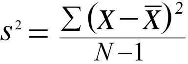
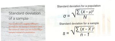
Descriptive Measures for Populations vs. Samples

Population parameters use Greek letters; sample statistics use Latin letters. For example:

Measure	Sample Statistic	Population Parameter
Mean	\( \bar{x} \)	\( \mu \)
Variance	\( s^2 \)	\( \sigma^2 \)
Standard Deviation	\( s \)	\( \sigma \)

Numerical Descriptive Measures

Standard Deviation and Variance

The formulas for standard deviation and variance differ for populations and samples:

• Population Standard Deviation: $\sigma = \sqrt{ \frac{ \sum (x - \mu)^2 }{ N } }$

• Sample Standard Deviation: $s = \sqrt{ \frac{ \sum (x - \bar{x})^2 }{ n - 1 } }$

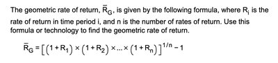
Geometric Mean and Rate of Return

The geometric mean is used for data combined multiplicatively, such as growth rates. The geometric rate of return is:

• $\bar{R}_G = \left[ (1 + R_1) (1 + R_2) \cdots (1 + R_n) \right]^{1/n} - 1$

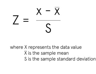
Z-Scores

A Z-score standardizes a data value by expressing it in terms of standard deviations from the mean:

• $Z = \frac{X - \bar{X}}{S}$

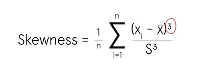
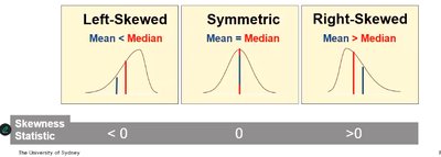
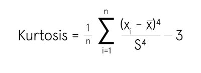
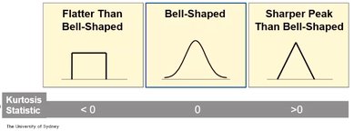
Skewness and Kurtosis

These statistics describe the shape of a distribution:

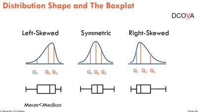
• Skewness: Measures asymmetry. Left-skewed (mean < median), right-skewed (mean > median), symmetric (mean = median).

• Kurtosis: Measures the concentration of values in the tails. High kurtosis indicates heavy tails; low kurtosis indicates light tails.

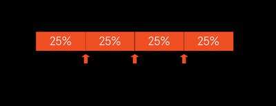
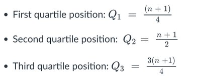
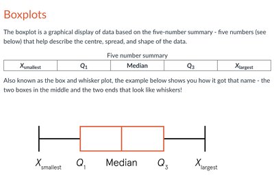
Quartiles, Interquartile Range, and Boxplots

Quartiles divide data into four equal parts. The interquartile range (IQR) measures the spread of the middle 50% of data:

• First Quartile (Q1): $Q_1 = \frac{n+1}{4}$

• Second Quartile (Median, Q2): $Q_2 = \frac{n+1}{2}$

• Third Quartile (Q3): $Q_3 = \frac{3(n+1)}{4}$

• IQR: $Q_3 - Q_1$

Probability and Probability Distributions

Basic Probability Concepts

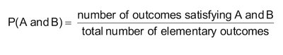
Probability quantifies the likelihood of an event, ranging from 0 (impossible) to 1 (certain). Events can be simple or joint, and probabilities can be assessed a priori, empirically, or subjectively.

• Marginal Probability: Probability of a single event.

• Joint Probability: Probability of two or more events occurring together.

• Conditional Probability: Probability of one event given another has occurred.

Probability Rules and Tables

Key probability rules include the addition rule, multiplication rule, and Bayes' theorem. Probabilities are often organized in contingency tables for clarity.

Event	B1	B2	Total
A1	P(A1 and B1)	P(A1 and B2)	P(A1)
A2	P(A2 and B1)	P(A2 and B2)	P(A2)
Total	P(B1)	P(B2)	1

Additional info:

• All formulas are provided in LaTeX format for clarity and academic rigor.

• Images are included only when directly relevant to the explanation and reinforce the educational content.