Ch. 25 Categorical Explanatory Variables in Regression: Two-Sample Comparisons, ANCOVA, and Multiple Groups

Study Guide - Smart Notes

Tailored notes based on your materials, expanded with key definitions, examples, and context.

Chapter 25: Categorical Explanatory Variables

25.1 Two-Sample Comparisons

When analyzing the effect of a categorical explanatory variable (such as diamond clarity grade) on a quantitative response (such as price), two-sample comparisons are often used. This section explores how to compare means between two groups and the statistical considerations involved.

Key Point 1: Categorical Explanatory Variables: These are variables that divide data into groups (e.g., VS1 vs. VVS1 diamond clarity grades).
Key Point 2: Two-Sample t-Test: Used to compare the means of two independent groups. The null hypothesis is that the group means are equal: .
Key Point 3: Conditions for Inference:
- No obvious lurking (confounding) variable explains the difference.
- Data are simple random samples (SRS).
- Groups have similar variances.
- Each sample meets the sample size condition (usually for each group).
Key Point 4: Statistical Significance: If the confidence interval for the difference in means does not include zero, the difference is statistically significant.
Example: The average price for VS1 diamonds is $1,095.9, and for VVS1 diamonds is $1,169. The observed difference ($73.10) is statistically significant if zero is not in the confidence interval.

Confounding Variables: A confounding variable (e.g., weight) is one that is related to both the explanatory and response variables, potentially biasing the results. To check for confounding, compare the means of the confounder between groups using a two-sample t-test.

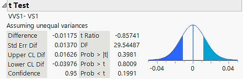
t-test output for weight comparison

Additional info: In the example, the p-value for the difference in weights between VS1 and VVS1 is high, so weight is not a confounder.

25.2 Analysis of Covariance (ANCOVA)

Analysis of Covariance (ANCOVA) extends regression by including both categorical and quantitative explanatory variables, allowing for adjustment for confounders and testing for interactions.

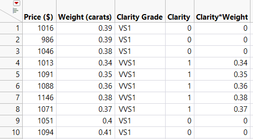
Key Point 1: Dummy Variables: Categorical variables are represented in regression by dummy (indicator) variables (e.g., Clarity = 1 for VVS1, 0 for VS1).
Key Point 2: Interaction Terms: The product of a dummy variable and a quantitative variable (e.g., Clarity × Weight) tests whether the effect of the quantitative variable differs by group.
Key Point 3: Model Interpretation: The coefficient for the dummy variable represents the difference in intercepts; the coefficient for the interaction term represents the difference in slopes between groups.
Example: Regression model for diamond price with Clarity, Weight, and Clarity × Weight as predictors.

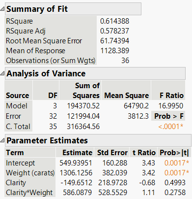
Data table with dummy and interaction variables Regression output for ANCOVA model

Additional info: The regression output shows parameter estimates for intercept, weight, clarity, and the interaction term. Statistical significance is assessed via p-values.

25.3 Checking Conditions

Before drawing inferences from regression or ANCOVA, it is essential to check model assumptions, particularly the assumption of similar variances across groups.

Key Point 1: Residual Plots: Plot residuals against fitted values to check for patterns or unequal spread.
Key Point 2: Boxplots of Residuals: Side-by-side boxplots for each group help assess variance similarity. If the interquartile range (IQR) for one group is more than twice that of another, the assumption is violated.

25.4 Interactions and Inference

Interactions in regression models allow the effect of one variable to depend on the level of another. Proper handling of interactions is crucial for valid inference.

Key Point 1: Principle of Marginality: If an interaction is statistically significant, retain it and both main effects in the model, regardless of their individual significance.
Key Point 2: Model Simplification: If the interaction is not significant, remove it for a simpler, more interpretable model (parallel lines for groups).
Key Point 3: Collinearity: Including interaction terms can increase collinearity, as measured by the Variance Inflation Factor (VIF).

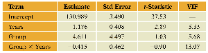
Regression table with interaction and VIF

Additional info: High VIF values indicate collinearity, which can inflate standard errors and complicate interpretation.

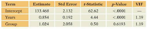
Regression table without interaction term

Additional info: Removing the non-significant interaction term simplifies the model and reduces VIF.

25.5 Regression with Several Groups

When the categorical explanatory variable has more than two groups, multiple dummy variables are used in regression. This allows for comparison among several groups while controlling for other variables.

Key Point 1: Dummy Variable Coding: For J groups, use J-1 dummy variables. The group with all dummies set to zero serves as the reference (baseline) group.
Key Point 2: Model Interpretation: Coefficients for dummy variables represent differences from the baseline group.
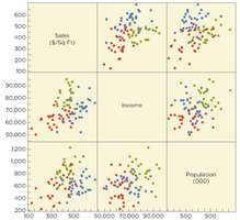
Key Point 3: Example Application: Estimating store sales using income, population, and market type (urban, suburban, rural) as predictors.

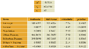
Scatterplot matrix for sales, income, and population by group Regression output for multiple groups

Example Equations:

Rural Stores (baseline):
Urban Stores:

Interpretation: Urban stores have higher baseline sales than rural stores, but the effect of income on sales is smaller in urban areas. The effect of population is constant across locations since there is no interaction term between population and location.