Chapter 10: Sampling Distributions – Study Notes for Business Statistics

Sampling Distributions

Introduction to Sampling Distributions

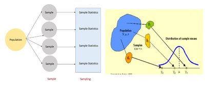
Sampling distributions are fundamental in statistical inference, allowing us to understand how sample statistics (such as means or proportions) behave when drawn from a population. The concept is crucial for estimating population parameters and assessing the reliability of sample results.

• Population: The entire group of individuals or items of interest.

• Sample: A subset of the population, selected according to a specific method.

• Sampling Error: The natural discrepancy between a sample statistic and the corresponding population parameter, calculated as $\bar{y} - \mu$.

Sampling Distribution of the Mean

Definition and Properties

The sampling distribution of the mean is the probability distribution of all possible sample means for samples of a given size drawn from a population. This distribution is central to inferential statistics.

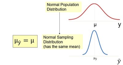
• Mean of Sampling Distribution: The mean of all sample means equals the population mean ($\mu_{\bar{y}} = \mu$), making the sample mean an unbiased estimator.

• Standard Deviation (Standard Error): The standard deviation of the sampling distribution of the mean is $\sigma_{\bar{y}} = \frac{\sigma}{\sqrt{n}}$, where $\sigma$ is the population standard deviation and $n$ is the sample size.

Cases for the Shape of the Sampling Distribution

• Case I (Normal Population, Known $\sigma$): If the population is normal, the sampling distribution of the mean is also normal for any sample size: $\bar{y} \sim N(\mu, \frac{\sigma}{\sqrt{n}})$.

• Case II (Normal Population, Unknown $\sigma$): If $\sigma$ is unknown, use the sample standard deviation $s$ and the distribution follows Student's t-distribution: $\bar{y} \sim t(\mu, \frac{s}{\sqrt{n}})$ with $n-1$ degrees of freedom.

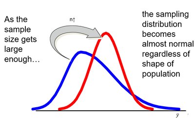
• Case III (Non-Normal Population, Large $n$): By the Central Limit Theorem (CLT), for large $n$ (typically $n \geq 30$), the sampling distribution of the mean is approximately normal regardless of the population's shape.

• Case IV (Non-Normal Population, Unknown $\sigma$, Large $n$): The sampling distribution of the mean follows a t-distribution using the CLT.

Student's t-Distribution

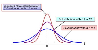
The t-distribution is used when the population standard deviation is unknown and the sample size is small. It is more variable than the normal distribution and has heavier tails. As the sample size increases, the t-distribution approaches the normal distribution.

• Degrees of Freedom (df): $df = n - 1$

• Heavier Tails: Accounts for extra variability due to estimating $\sigma$ with $s$.

The Central Limit Theorem (CLT)

Statement and Importance

The Central Limit Theorem states that, for a sufficiently large sample size, the sampling distribution of the sample mean will be approximately normal, regardless of the population's distribution. This theorem justifies the use of normal probability models in many practical situations.

• Sample Size Rule: A common rule is $n \geq 30$ for the CLT to apply.

• Symmetric Populations: Smaller samples may suffice if the population is symmetric.

• Highly Skewed Populations: Larger samples are needed for the sampling distribution to be normal.

Examples of CLT in Action

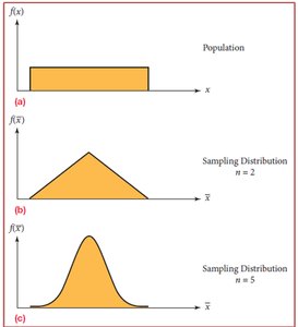
• Uniform Population: Even with a non-normal (uniform) population, the sampling distribution of the mean becomes normal as $n$ increases.

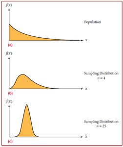
• Triangular and Skewed Populations: The same principle applies; the sampling distribution of the mean becomes more normal with larger $n$.

Assumptions and Conditions for Sampling Distributions

• Independence: Sampled values must be independent.

• Randomization: Data must be randomly sampled.

• 10% Condition: Sample size should be no more than 10% of the population when sampling without replacement. If violated, apply the finite population correction factor (FPCF).

• Large Enough Sample Condition: For highly skewed populations, larger samples are needed for the sampling distribution to be approximately normal.

Standard Error and Finite Population Correction

Standard Error Formulas

• Known $\sigma$: $\sigma_{\bar{y}} = \frac{\sigma}{\sqrt{n}}$

• Unknown $\sigma$: $\sigma_{\bar{y}} = \frac{s}{\sqrt{n}}$

• With FPCF (if $n/N > 0.10$): $\sigma_{\bar{y}} = \frac{\sigma}{\sqrt{n}} \sqrt{\frac{N-n}{N-1}}$ or $\sigma_{\bar{y}} = \frac{s}{\sqrt{n}} \sqrt{\frac{N-n}{N-1}}$

Sampling Distribution of Proportions

Population and Sample Proportions

• Population Proportion ($p$): $p = \frac{Y}{N}$, where $Y$ is the number of items with the attribute in the population, $N$ is the population size.

• Sample Proportion ($\hat{p}$): $\hat{p} = \frac{y}{n}$, where $y$ is the number of items with the attribute in the sample, $n$ is the sample size.

Sampling Distribution of Proportions

• Mean: $\mu_{\hat{p}} = p$

• Standard Error: $\sigma_{\hat{p}} = \sqrt{\frac{pq}{n}}$, where $q = 1 - p$

• Shape: For large $n$, the distribution is approximately normal; for small $n$, it is binomial.

Conditions for Normal Approximation

• Independence and Randomization

• 10% Condition

• Success/Failure Condition: $np \geq 10$ and $nq \geq 10$

Standard Error with Finite Population Correction

• With FPCF: $\sigma_{\hat{p}} = \sqrt{\frac{pq}{n}} \sqrt{\frac{N-n}{N-1}}$

Calculating Probabilities for Sample Means and Proportions

Sample Means

• Direct Scenario: Given $\bar{y}$, calculate $z = \frac{\bar{y} - \mu}{\sigma_{\bar{y}}}$ or $t = \frac{\bar{y} - \mu}{s/\sqrt{n}}$

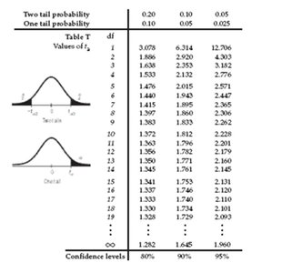
• Working Backward: Given probability, find $z$ or $t$ from tables, then solve for $\bar{y}$.

Sample Proportions

• Direct Scenario: Given $\hat{p}$, calculate $z = \frac{\hat{p} - p}{\sigma_{\hat{p}}}$

• Working Backward: Given probability, find $z$ from tables, then solve for $\hat{p}$.

Summary Table: Key Formulas

Statistic	Mean	Standard Error (10% Condition Satisfied)	Standard Error (FPCF Applied)
Sample Mean ($\bar{y}$, $\sigma$ known)	$\mu$	$\frac{\sigma}{\sqrt{n}}$	$\frac{\sigma}{\sqrt{n}} \sqrt{\frac{N-n}{N-1}}$
Sample Mean ($\bar{y}$, $\sigma$ unknown)	$\mu$	$\frac{s}{\sqrt{n}}$	$\frac{s}{\sqrt{n}} \sqrt{\frac{N-n}{N-1}}$
Sample Proportion ($\hat{p}$)	$p$	$\sqrt{\frac{pq}{n}}$	$\sqrt{\frac{pq}{n}} \sqrt{\frac{N-n}{N-1}}$

Practice and Application

• Use the formulas and tables to calculate probabilities and critical values for sample means and proportions.

• Always check assumptions and conditions before applying normal or t-distribution approximations.