Chapter 17: Comparison – Statistical Methods for Comparing Groups

Chapter 17: Comparison

17.1 Data for Comparisons

Comparing two groups is a fundamental task in business statistics, often used to evaluate the effectiveness of different treatments, products, or strategies. Inferential statistics allow us to test for differences between two populations using sample data.

• Key Point 1: Framing the Comparison: Define the parameter of interest (e.g., difference in proportions or means) and set up hypotheses to test whether a meaningful difference exists.

• Key Point 2: Example – Diet Comparison: Suppose a fitness chain wants to know if a proprietary diet leads to higher membership renewal rates than a conventional diet. Let pA be the proportion renewing on the Atkins diet, and pC for the conventional diet. The difference pA - pC measures the effect.

• Key Point 3: Hypotheses: For profitability, the chain requires the difference to exceed 4%. $H_0: p_A - p_C \leq 0.04$ $H_A: p_A - p_C > 0.04$

• Key Point 4: Confounding: Confounding occurs when the effects of multiple factors are mixed, making it difficult to attribute differences to the treatment alone. Randomization helps eliminate confounding. If randomization is not possible, ensure independent sampling from each population.

Summary Statistics – Diet Comparison

Summary statistics and confidence intervals are used to compare the two groups. Overlapping confidence intervals suggest no significant difference, while non-overlapping intervals indicate a statistically significant difference.

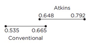
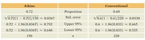
• Example: The 95% confidence interval for the difference in renewal proportions (Atkins vs. Conventional) is (0.023, 0.217), which does not include zero. This suggests a statistically significant difference in renewal rates.

Interpreting the Confidence Interval

If the confidence interval for the difference between two proportions (or means) does not include zero, we conclude that the groups are statistically significantly different at the chosen confidence level (typically 95%).

• Application: Members on the Atkins diet renew at a statistically significantly higher rate than those on the conventional diet.

17.2 Two-Sample t-Test

Comparing Means of Two Independent Groups

The two-sample t-test is used to compare the means of two independent groups. This test is appropriate when the outcome variable is quantitative and the groups are independent.

• Key Point 1: Hypotheses: $H_0: \mu_1 - \mu_2 \leq D_0$ $H_1: \mu_1 - \mu_2 > D_0$ where $\mu_1$ and $\mu_2$ are the population means for groups 1 and 2, and $D_0$ is the hypothesized difference (often zero).

• Key Point 2: Example – Used Car Prices: Let $\mu_1$ be the mean price of used four-wheel drive luxury cars, and $\mu_2$ for two-wheel drive. The test checks if four-wheel drive models command a higher price.

• Key Point 3: Checklist for Validity:

  • No obvious lurking variables

  • Simple random samples (SRS)

  • Similar variances (though the test can accommodate unequal variances)

  • Adequate sample size

95% Confidence Interval for the Difference in Means

The confidence interval for $\mu_1 - \mu_2$ provides a range of plausible values for the difference in population means. If the interval does not include zero, the means are statistically significantly different.

• Interpretation: In the example, the 95% confidence interval for the difference in mean prices does not include zero, indicating a significant difference between the two types of cars.

Practice Question: Matched Pairs t-Test

Comparing Paired Data

When comparing two measurements from the same subjects (e.g., sales in 2015 and 2016 for the same stores), a matched pairs t-test is appropriate. This test accounts for the pairing and focuses on the differences within each pair.

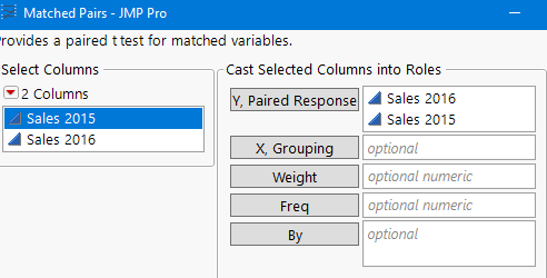
• Key Point 1: Application: The sales volume (in dollars per square foot) for 86 retail outlets is compared between 2015 and 2016 to determine if there was a statistically significant change.

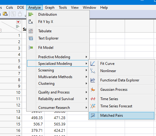
• Key Point 2: Software Steps: In JMP, use Analyze → Specialized Modeling → Matched Pairs to conduct the test.

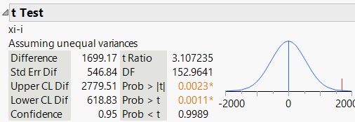
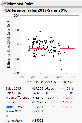
Interpreting the Results

The 95% confidence interval for the mean difference is (−27.85, −9.84). Since this interval does not include zero, there is sufficient evidence to conclude that sales changed by a statistically significant amount from 2015 to 2016 (at α = 0.05).

• Formula for Paired t-Test: $t = \frac{\overline{d}}{s_d / \sqrt{n}}$ where $\overline{d}$ is the mean of the differences, $s_d$ is the standard deviation of the differences, and $n$ is the number of pairs.

Additional info: The notes above expand on the original slides by providing definitions, formulas, and context for the statistical tests discussed. The images included are directly relevant to the statistical concepts and reinforce the explanations provided.