Chapter 21: The Simple Regression Model – Business Statistics Study Notes

The Simple Regression Model (SRM)

Introduction to Simple Regression

The Simple Regression Model (SRM) is a foundational statistical tool used to describe the relationship between a single explanatory variable (X) and a response variable (Y). In business statistics, SRM helps answer questions such as how order size affects production time or how advertising spending influences sales.

• Definition: SRM models the association between an explanatory variable and a response variable in a population.

• Purpose: To estimate and infer the conditional mean of Y given X.

• Equation: The SRM is typically written as $Y = \beta_0 + \beta_1 X + \varepsilon$, where $\varepsilon$ is the error term.

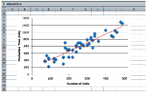
• Example: Estimated Production Time = 172 + 2.44 × Number of Units

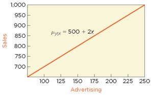
Linear on Average

The SRM describes how the conditional mean of Y depends linearly on X. The regression line is characterized by an intercept ($\beta_0$) and a slope ($\beta_1$).

• Conditional Mean: $\mu_{Y|X} = \beta_0 + \beta_1 X$

• Interpretation: The regression line represents the average response for each value of X.

Deviations from the Mean (Errors)

Observed values of Y deviate from the regression line due to random errors ($\varepsilon$). These errors are assumed to have certain properties:

• Independence: Errors are independent of each other.

• Equal Variance: All errors have the same variance ($\text{Var}(\varepsilon) = \sigma^2$).

• Normality: Errors are normally distributed.

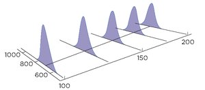
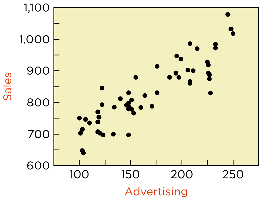
Data Generating Process

The SRM assumes that for each value of X, the response Y is normally distributed around the regression line. The true regression line is a characteristic of the population, not the observed data.

• Population Model: $Y = \beta_0 + \beta_1 X + \varepsilon$, $\varepsilon \sim N(0, \sigma^2)$

• Observed Data: Data points are sampled from this population model.

Conditions for the SRM

Checklist for Validity

Before applying SRM, certain conditions must be checked to ensure the model's validity:

• Linearity: Is the association between Y and X linear?

• Equal Variance: Are the variances of the residuals similar?

• Lurking Variables: Have we ruled out other variables that might affect the relationship?

• Independence: Are the errors independent?

• Normality: Are the residuals nearly normal?

Production Time Example

In the production time example, the conditions for SRM are illustrated:

• Linearity: No pattern in the residuals.

• Equal Variance: Spread of residuals is constant around the horizontal line.

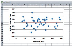
• Lurking Variables: No obvious lurking variable, but context matters (e.g., complexity of parts).

• Independence: No evidence that one run influences another.

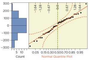
• Normality: Nearly normal condition satisfied; otherwise, rely on the Central Limit Theorem (CLT) for large samples.

Modeling Process

The process for fitting and validating an SRM includes:

• Plot Y versus X to verify linearity.

• Fit the least squares regression line.

• Plot and inspect residuals for patterns.

• Construct a time plot of residuals if data are time series.

• Inspect the quantile plot of residuals for normality.

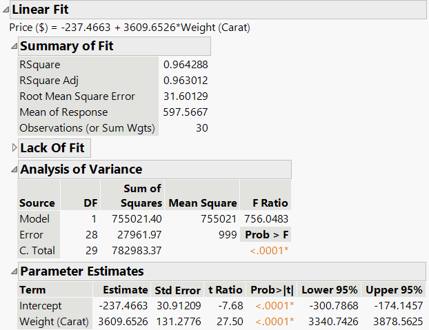
Inference in Regression

Parameters and Estimates

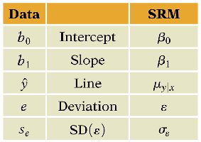
SRM involves estimating parameters and making inferences about them. The table below summarizes the correspondence between data and SRM terms:

Data	SRM
b0	Intercept (β0)
b1	Slope (β1)
ŷ	Line (μY|X)
e	Deviation (ε)
se	SD(ε) (σε)

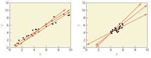
Standard Errors

Standard errors measure the sample-to-sample variability of the estimated intercept (b0) and slope (b1). The estimated standard error of b1 is influenced by:

• Standard deviation of the residuals: Higher residual SD increases standard error.

• Sample size: Larger sample size decreases standard error.

• Standard deviation of X: Greater spread in X increases standard error.

Hypothesis Tests in Regression

Hypothesis tests are used to determine if the intercept or slope is significantly different from zero:

• Test for Intercept: H0: β0 = 0 vs. HA: β0 ≠ 0

• Test for Slope: H0: β1 = 0 vs. HA: β1 ≠ 0

• t-statistic: Used to assess significance; large absolute values and small p-values indicate significance.

Confidence Intervals

Confidence intervals provide a range of plausible values for regression parameters. A 95% confidence interval for β0 or β1 is calculated as:

• $\text{Estimate} \pm t^* \times \text{Standard Error}$

• If zero lies outside the interval, the parameter is significantly different from zero.

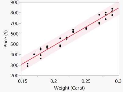
Prediction Intervals

Leveraging the SRM for Prediction

A prediction interval is designed to hold a fraction (usually 95%) of the values of the response for a given value of X. Unlike confidence intervals, prediction intervals make statements about new observations rather than population parameters.

• Approximate Formula: $\hat{Y} \pm t^* \times \text{Standard Error}_{\text{pred}}$

• Prediction intervals are reliable within the range of observed data and sensitive to assumptions of constant variance and normality.

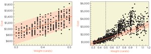
Reliability and Limitations

Prediction intervals fail when the SRM does not hold, especially in cases of extrapolation beyond the observed data range.

Summary Table: SRM Terms and Data

Term	Meaning
β0	Population Intercept
β1	Population Slope
b0	Sample Intercept Estimate
b1	Sample Slope Estimate
ε	Error (Deviation from Mean)
σε	Standard Deviation of Errors

Additional info: These notes expand on brief points from the original slides, providing definitions, formulas, and examples for clarity and completeness. All images included are directly relevant to the explanation of the adjacent paragraph, reinforcing key concepts in the SRM chapter.