Chapter 22: Regression Diagnostics – Business Statistics Study Notes

Regression Diagnostics

Introduction

Regression diagnostics are essential for evaluating the validity and reliability of regression models in business statistics. This chapter focuses on three main issues: changing variation (heteroscedasticity), outliers, and dependent errors (autocorrelation), and provides methods for detecting and addressing these problems.

Changing Variation

Understanding Changing Variation

In regression analysis, the variability of the response variable may change across levels of the explanatory variable. This is particularly evident in cases such as home prices, where larger homes tend to have more variable prices.

• Heteroscedasticity: Errors have different amounts of variation across levels of the explanatory variable.

• Homoscedasticity: Errors have equal amounts of variation.

• Implications: Violating the similar variances condition affects the reliability of confidence intervals and hypothesis tests.

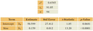
Example: Home Price vs. Size

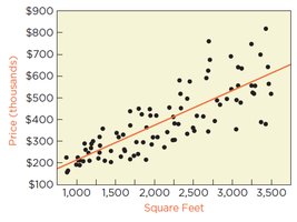
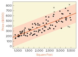
Scatterplots and residual plots can reveal changing variation. In the home price example, both the mean and standard deviation of price increase with home size.

Detecting Changing Variation

• Scatterplot: Shows increasing spread of prices with home size.

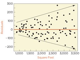
• Residual Plot: Fan-shaped pattern indicates heteroscedasticity.

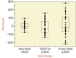
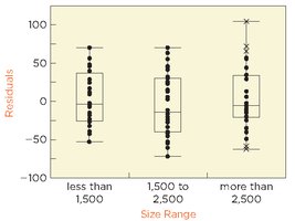
• Boxplots: Side-by-side boxplots of residuals by size range confirm increasing variance.

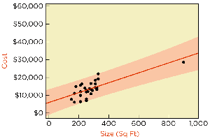
Consequences of Heteroscedasticity

• Prediction intervals may be too narrow or too wide.

• Confidence intervals for slope and intercept are unreliable.

• Hypothesis tests for coefficients may be invalid.

Fixing Changing Variation

One solution is to revise the model by transforming the response variable. For example, dividing price by square feet and using the reciprocal of square feet as the explanatory variable can stabilize variance.

• Transformed Model: Response variable becomes price per square foot; explanatory variable is reciprocal of square feet.

• Result: Residuals exhibit similar variances (homoscedasticity).

Comparing Models

Although the revised model may have a lower $r^2$, it provides more reliable confidence and prediction intervals.

Outliers

Identifying Outliers

Outliers are observations that deviate markedly from the pattern of the data. In regression, outliers can have high leverage, meaning they strongly influence the regression line.

• Leverage: An observation with an extreme value of the explanatory variable.

• Impact: Outliers can distort estimates of regression coefficients and prediction intervals.

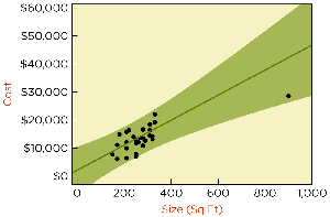
Example: Contractor's Bid

In a dataset of contractor bids, one project at 900 square feet is an outlier and a leveraged observation.

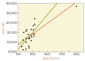
Consequences of Outliers

• Including the outlier shifts the estimated fixed cost and marginal cost by more than one standard error.

• Prediction intervals change significantly depending on whether the outlier is included.

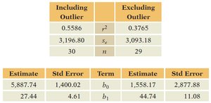
Handling Outliers

• Decide whether to include or exclude the outlier based on whether it represents expected future conditions.

• Gather more information to make an informed decision.

Dependent Errors and Time Series

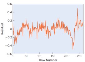
Detecting Dependence

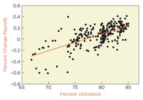
In time series data, errors may be correlated across time, violating the independence assumption. This is known as autocorrelation.

• Durbin-Watson Statistic: Tests for autocorrelation in residuals.

• Null Hypothesis: Adjacent residuals are uncorrelated ($H_0: \rho_e = 0$).

• Interpretation: If D is approximately 2, residuals are uncorrelated.

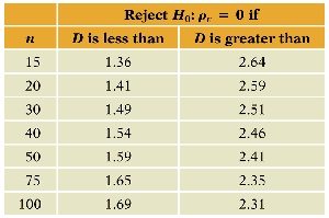
Durbin-Watson Statistic

• Use p-value or critical values to determine if autocorrelation is present.

• Critical values table helps decide when to reject the null hypothesis.

Consequences of Dependence

• Positive autocorrelation leads to underestimated standard errors.

• Estimated slope and intercept are less precise.

• Best remedy: Incorporate dependence into the regression model (e.g., using time series models).

Key Terms and Formulas

• Heteroscedasticity: Unequal variance of errors.

• Homoscedasticity: Equal variance of errors.

• Leverage: Influence of an observation on the regression line.

• Autocorrelation: Correlation of residuals across time.

• Durbin-Watson Statistic: $D = \frac{\sum_{t=2}^{n} (e_t - e_{t-1})^2}{\sum_{t=1}^{n} e_t^2}$

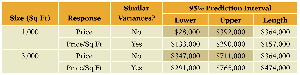
Summary Table: Model Comparison

The following tables summarize the comparison between models with and without variance stabilization, and the impact of outliers:

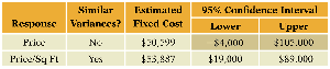
Response	Similar Variances?	Estimated Fixed Cost	95% Confidence Interval Lower	Upper
Price	No	$50,599	$4,000	$105,000
Price/Sq Ft	Yes	$53,887	$19,000	$88,000

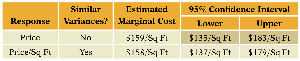
Response	Similar Variances?	Estimated Marginal Cost	95% Confidence Interval Lower	Upper
Price	No	$159/Sq Ft	$135/Sq Ft	$183.5/Sq Ft
Price/Sq Ft	Yes	$0.159/Sq Ft	$0.137/Sq Ft	$0.179/Sq Ft

Size (Sq Ft)	Response	Similar Variances?	95% Prediction Interval Lower	Upper	Length
1,000	Price	No	$238,000	$382,000	$144,000
1,000	Price/Sq Ft	Yes	$153,000	$206,000	$53,000
3,000	Price	No	$367,000	$781,000	$414,000
3,000	Price/Sq Ft	Yes	$501,000	$546,000	$45,000

n	D is less than	D is greater than
15	1.36	2.64
20	1.41	2.59
30	1.49	2.51
40	1.54	2.46
50	1.59	2.41
75	1.65	2.35
100	1.69	2.31

Additional info: Academic context and explanations have been expanded for clarity and completeness. All images included are directly relevant to the adjacent content and reinforce key concepts.