Chapter 23: Multiple Regression – Business Statistics Study Notes

Multiple Regression Model

Introduction to Multiple Regression

Multiple regression is a statistical technique used to model the relationship between a response variable and two or more explanatory variables. It allows researchers to separate the effects of each explanatory variable and determine which variables significantly impact the response.

• Definition: The multiple regression model (MRM) describes the association in the population between multiple explanatory variables and a response.

• Equation: The response variable Y is linearly related to k explanatory variables X1, X2, ..., Xk by the equation: $Y = \beta_0 + \beta_1 X_1 + \beta_2 X_2 + \ldots + \beta_k X_k + \varepsilon$ where $\varepsilon \sim N(0, \sigma^2)$ (errors are independent, have equal variance, and are normally distributed).

• Comparison: Simple regression bundles all but one explanatory variable into the error term, while multiple regression includes several variables in the model.

• Residuals: Departures from normality in residuals may indicate omitted explanatory variables.

Interpreting Multiple Regression

Example: Women’s Apparel Stores

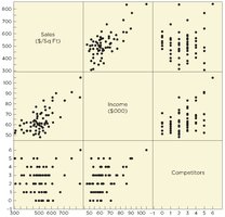
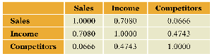
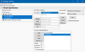
This example models annual sales per square foot in a chain of women’s apparel stores using two explanatory variables: median household income in the area and the number of competing apparel stores in the same mall.

• Scatterplot Matrix: Used to visualize relationships between variables before fitting the model.

• Correlation Matrix: Quantifies the strength and direction of linear relationships between variables.

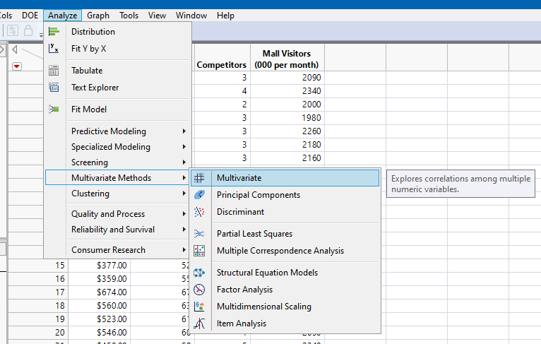
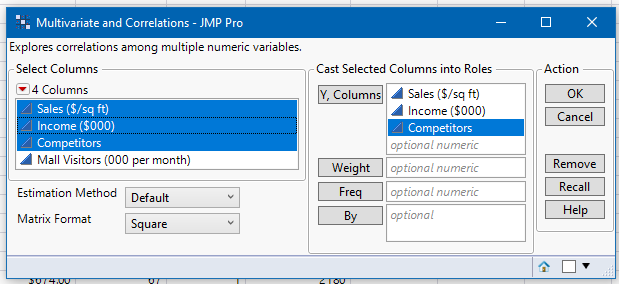
Fitting the Model

To fit the model, select the response and explanatory variables in statistical software.

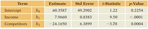
Model Equation and Interpretation

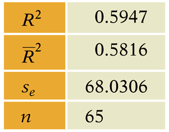
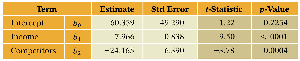
• Fitted Model: $\text{Sales} = 60.359 + 7.966 \times \text{Income} - 24.165 \times \text{Competitors}$

• R-squared ($R^2$): Indicates the proportion of variance in sales explained by the model. Here, $R^2 = 0.5947$ (59.47%).

• Adjusted R-squared: Adjusts for sample size and number of variables; always less than $R^2$.

• Standard error ($s_e$): Measures the average distance that the observed values fall from the regression line. Here, $s_e = 68.03$.

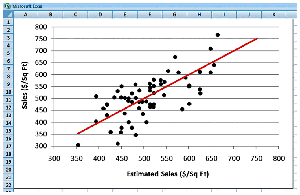
Calibration Plot

A calibration plot compares observed sales to fitted values. The tighter the data cluster along the diagonal, the higher the $R^2$.

Marginal and Partial Slopes

• Partial Slope: The slope of an explanatory variable in multiple regression, controlling for other variables.

• Marginal Slope: The slope in simple regression, not controlling for other variables.

• Interpretation: Partial and marginal slopes only agree when explanatory variables are uncorrelated.

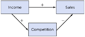
Path Diagram and Collinearity

• Path Diagram: Schematic drawing showing direct and indirect effects among variables.

• Collinearity: High correlations among explanatory variables can make estimates unreliable.

Checking Conditions for Inference

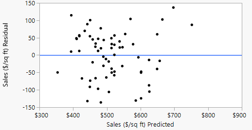
Residual Plots

Residual plots are used to check model assumptions: independence, equal variance, and normality of errors.

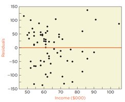
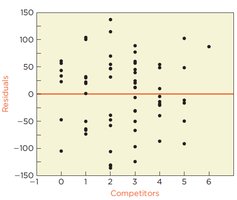
• Residuals vs. Fitted Values: Used to identify outliers and check for equal variance.

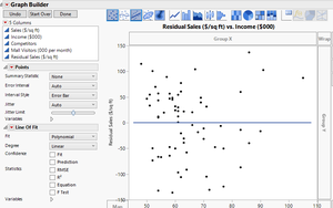
• Residuals vs. Explanatory Variables: Used to verify linear relationships.

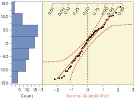
Normality Check

Normal quantile plots and histograms are used to check if residuals are approximately normally distributed.

Inference in Multiple Regression

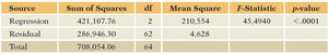
F-test for Model

The F-test evaluates the explanatory power of the model as a whole. The F-statistic is the ratio of the variance explained by the model to the variance of the residuals.

• Null Hypothesis ($H_0$): All slopes are equal to zero.

• Interpretation: A low p-value indicates that the model explains significant variation in the response.

Inference for Individual Coefficients

The t-test is used to test whether each slope is significantly different from zero.

• Null Hypothesis ($H_0$): $\beta_j = 0$ for each coefficient.

• Interpretation: Significant t-statistics and low p-values indicate that the explanatory variable has a significant effect.

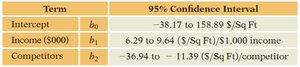
Confidence Intervals

Confidence intervals provide a range of plausible values for each coefficient, consistent with t-test results.

Prediction Intervals

A prediction interval estimates the range in which a new observation is likely to fall, given specific values of the explanatory variables. For example, a 95% prediction interval for sales at a location with median income of $70,000 and 3 competitors is $545.48 \pm $137.29 per square foot.

Steps in Fitting a Multiple Regression

Step-by-Step Process

1. Define the Problem: Identify the response and explanatory variables relevant to the business question.

2. Visualize Relationships: Use scatterplot matrices to check for linear relationships.

3. Fit the Model: If relationships are linear, fit the multiple regression model; otherwise, consider transformations.

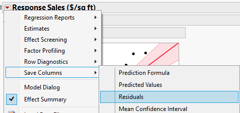
4. Check Residuals: Obtain residuals and fitted values, and make scatterplots to check for equal variance and dependence.

5. Check Normality: Use quantile plots and histograms to verify normality of residuals.

6. Test Model Significance: Use the F-statistic to test if explanatory variables collectively affect the response.

7. Interpret Partial Slopes: If the F-statistic is significant, interpret individual partial slopes and their confidence intervals.