Chapter 8: Randomness and Probability - Business Statistics Study Notes

Randomness and Probability

Introduction to Probability

Probability is a fundamental concept in statistics, representing the likelihood that a particular event will occur. In business statistics, probability helps managers make informed decisions based on uncertain outcomes. Probability values range from 0 (impossible event) to 1 (certain event).

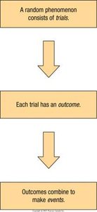
• Event: A specific outcome or a set of outcomes from a random phenomenon.

• Trial: Each attempt to observe a random phenomenon.

• Outcome: The result of a single trial.

• Sample Space (S or Ω): The set of all possible outcomes.

Types of Probability

There are three main methods for estimating probability:

• Empirical Probability: Based on observed data and long-run relative frequencies. Calculated as the number of times an event occurs divided by the total number of trials.

• Theoretical Probability: Calculated when all outcomes are equally likely. Formula: $P(A) = \frac{\text{Number of outcomes in } A}{\text{Total number of outcomes}}$

• Subjective Probability: Based on personal judgment or experience, not on data or equally likely outcomes. Subjective probability is prone to biases such as overconfidence, sunk cost, and recency bias.

Law of Large Numbers (LLN)

The Law of Large Numbers states that as the number of independent trials increases, the empirical probability (long-run relative frequency) of an event approaches its true probability. This principle is essential for making reliable statistical inferences from sample data.

• Key Point: The Law of Averages (the idea that things must even out in the short run) does not exist.

Probability Rules

Basic Probability Rules

• Rule 1: Probability of any event is between 0 and 1: $0 \leq P(A) \leq 1$

• Rule 2 (Probability Assignment Rule): The probability of the sample space is 1: $P(S) = 1$

• Rule 3 (Complement Rule): $P(A^C) = 1 - P(A)$, where $A^C$ is the complement of event A.

• Rule 4 (Multiplication Rule for Independent Events): $P(A \text{ and } B) = P(A) \times P(B)$, if A and B are independent.

• Rule 5 (Addition Rule for Disjoint Events): $P(A \text{ or } B) = P(A) + P(B)$, if A and B are disjoint.

• Rule 6 (General Addition Rule): $P(A \text{ or } B) = P(A) + P(B) - P(A \text{ and } B)$

Joint, Marginal, and Conditional Probability

Contingency Tables

Contingency tables organize data to show the frequency or probability of combinations of events. They are useful for calculating joint, marginal, and conditional probabilities.

Gender	Skis	Camera	Bike	Total
Man	117	50	60	227
Woman	130	91	30	251
Total	247	141	90	478

• Marginal Probability: Probability based on totals in the margins (e.g., $P( ext{woman}) = \frac{251}{478} = 0.525$).

• Joint Probability: Probability of two events occurring together (e.g., $P( ext{woman and camera}) = \frac{91}{478} = 0.190$).

• Conditional Probability: Probability of one event given another (e.g., $P( ext{bike} | ext{woman}) = \frac{30}{251} = 0.120$).

Conditional Probability and Independence

Conditional probability is written as $P(B|A)$, meaning the probability of B given A. Independence means the occurrence of one event does not affect the probability of another.

• General Multiplication Rule: $P(A \text{ and } B) = P(A) \times P(B|A)$

• Independence: Events A and B are independent if $P(B|A) = P(B)$

• Disjoint vs. Independent: Disjoint events cannot be independent.

Constructing Contingency Tables

Example: Housing Survey

Given probabilities, you can construct a contingency table to find other probabilities. For example, if 56% of houses have at least 2 bathrooms, 62% are low priced, and 22% are both, the table is:

Price	At Least Two Bathrooms (True)	At Least Two Bathrooms (False)	Total
Low	0.22	0.40	0.62
High	0.34	0.04	0.38
Total	0.56	0.44	1.00

Additional info: Probabilities in the table add up to marginal totals, and the cells represent disjoint events.

Probability Trees

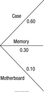
Tree Diagrams for Probability

Probability trees visually represent the sequence of events and their probabilities, including conditional probabilities. They are useful for calculating joint probabilities and updating estimates.

• Branches: Represent different possible outcomes or events.

• Conditional Probabilities: Probabilities that depend on previous outcomes.

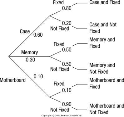
Example Calculation: Probability that a case adjustment fixes the problem: $P( ext{Case and Fixed}) = P( ext{Case}) \times P( ext{Fixed} | ext{Case}) = 0.60 \times 0.80 = 0.48$

Bayes's Rule

Reversing Conditioning and Updating Probabilities

Bayes's Rule allows us to update probability estimates given new information and to reverse conditioning. It is especially useful when calculating the probability of an initial event given the outcome.

• Bayes's Rule Formula: $P(A_i | B) = \frac{P(B | A_i) \times P(A_i)}{\sum_{j=1}^n P(B | A_j) \times P(A_j)}$

• Application: Used to update beliefs or probabilities as new data becomes available.

Common Pitfalls in Probability

• Probabilities must add up to 1 for all possible outcomes.

• Only add probabilities for disjoint events.

• Only multiply probabilities for independent events.

• Do not confuse disjoint and independent events.

Summary of Key Concepts

• Probability is based on long-run relative frequencies.

• The Law of Large Numbers applies to long-run behavior, not short-run averages.

• Probability can be estimated empirically, theoretically, or subjectively.

• Basic rules help combine probabilities for complex events.

• Independence and disjointness are distinct concepts.

• Probability trees and Bayes's Rule are tools for updating and calculating probabilities.