Ch. 18 Chi-Squared Tests: Inference for Counts in Business Statistics

Chi-Squared Tests: Inference for Counts

Introduction

Chi-squared tests are fundamental tools in business statistics for analyzing categorical data. They allow researchers to test hypotheses about relationships between categorical variables and the distribution of counts across categories. This chapter focuses on two main types of chi-squared tests: the test of independence and the test of goodness of fit.

Chi-Squared Test of Independence

Contingency Tables

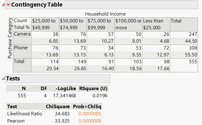
A contingency table displays the frequency counts of two categorical variables. In business contexts, such tables are used to examine relationships, such as whether household income affects the type of product purchased (e.g., camera or phone).

• Rows: Categories of one variable (e.g., purchase category)

• Columns: Categories of another variable (e.g., household income)

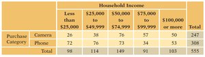
Example: The table below shows counts of camera and phone purchases across different income levels.

Purchase Category	Less than $25,000	$25,000 to $49,999	$50,000 to $74,999	$75,000 to $99,999	$100,000 or more	Total
Camera	26	38	76	57	50	247
Phone	72	76	73	34	53	308
Total	98	114	149	91	103	555

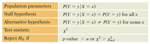
Hypotheses for the Chi-Squared Test

The test of independence evaluates whether two categorical variables are independent.

• Null Hypothesis (H0): The variables are independent (e.g., household income and purchase category are independent).

• Alternative Hypothesis (Ha): The variables are not independent.

Formally, for each income segment, the probability of purchasing a phone or camera is equal if H0 holds.

Calculating the Chi-Squared Statistic

The chi-squared statistic ($\chi^2$) measures the difference between observed and expected counts under the null hypothesis. Expected counts are calculated assuming independence, using the marginal totals of the contingency table.

• Formula: $\chi^2 = \sum \frac{(O - E)^2}{E}$, where O = observed count, E = expected count.

• Expected counts: For each cell, $E = \frac{(row\ total) \times (column\ total)}{grand\ total}$

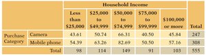
Example: Expected counts for each cell if variables are independent:

Purchase Category	Less than $25,000	$25,000 to $49,999	$50,000 to $74,999	$75,000 to $99,999	$100,000 or more	Total
Camera	43.61	50.74	66.31	40.50	45.84	247
Mobile phone	54.39	63.26	82.69	50.50	57.16	308
Total	98	114	149	91	103	555

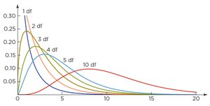
The Chi-Squared Distribution

The sampling distribution of the chi-squared statistic is right-skewed and defined only for positive values. The shape depends on the degrees of freedom (df), which increase with the size of the contingency table. As df increases, the distribution approaches normality.

• Degrees of freedom: $df = (r - 1)(c - 1)$, where r = number of rows, c = number of columns.

Interpreting Results: p-value and Decision

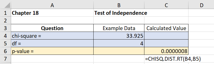
The p-value is the probability of observing a chi-squared statistic as extreme as the one calculated, assuming the null hypothesis is true. If p-value < significance level (α, typically 0.05), reject H0.

• Example: For the retail data, $\chi^2 = 33.925$, df = 4, p-value = 0.0000008.

• Decision: Since p < 0.05, reject H0. There is evidence that household income and purchase category are not independent.

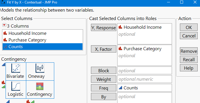
Software Application: JMP Example

Statistical software such as JMP can be used to perform chi-squared tests efficiently. The process involves selecting the relevant columns and specifying the roles for analysis.

Checklist for Valid Chi-Squared Test

• No obvious lurking variable

• Simple random sample (SRS) condition

• Contingency table condition

• Sample size condition: Expected cell frequencies at least 10; frequencies of 5 permitted with at least 4 df

Connection to Two-Sample Tests

The chi-squared test of independence is related to the two-sample test for proportions. If the confidence interval for the difference in proportions does not include zero, the chi-squared test will likely reject H0.

General Versus Specific Hypotheses

Limitations of the Chi-Squared Test

The chi-squared test is general and does not specify how proportions differ when H0 is rejected. More specific tests may have greater power to detect particular differences.

Chi-Squared Test of Goodness of Fit

Purpose and Hypotheses

The goodness of fit test evaluates whether observed counts for a single categorical variable match a specified probability distribution. The null hypothesis specifies expected counts based on a probability model (e.g., uniform distribution).

• Null Hypothesis (H0): The observed counts follow the specified distribution.

• Alternative Hypothesis (Ha): The observed counts do not follow the specified distribution.

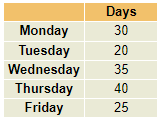
Example: Testing for Randomness

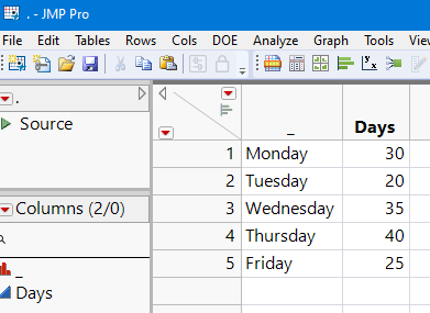
Suppose we want to test if employee absences are uniformly distributed across weekdays.

Day	Days
Monday	30
Tuesday	20
Wednesday	35
Thursday	40
Friday	25

Degrees of Freedom for Goodness of Fit

Degrees of freedom for the goodness of fit test are calculated as:

• $df = k - 1 -$ number of estimated parameters

• For 5 categories and no estimated parameters: $df = 5 - 1 = 4$

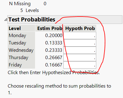
Expected Counts Under Uniform Distribution

If the null hypothesis assumes a uniform distribution, the expected count for each weekday is:

• Total days = 150

• Expected count per day = $150 / 5 = 30$

Calculating the Chi-Squared Statistic

Use the formula $\chi^2 = \sum \frac{(O - E)^2}{E}$ to compare observed and expected counts.

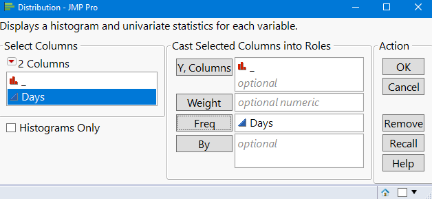
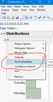
Software Application: JMP Example

JMP can be used to perform the goodness of fit test by entering observed counts and hypothesized probabilities.

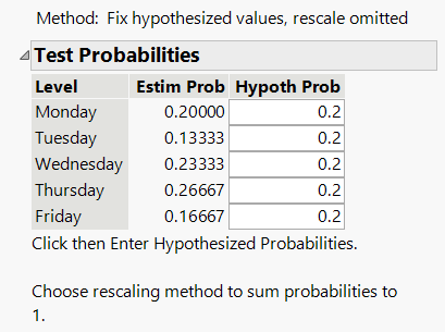
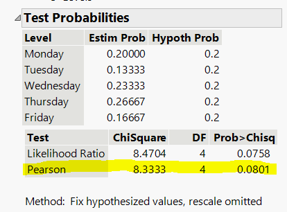
Interpreting Results

• Pearson ChiSquare: 8.33

• Degrees of freedom: 4

• p-value: 0.0801

• Decision: Since p > 0.05, do not reject H0. There is no evidence that absences are not uniformly distributed across weekdays.

Summary Table: Chi-Squared Test Components

Population parameters	Null hypothesis	Alternative hypothesis	Test statistic	Reject H0 if
P(Y = y | X = x)	P(Y = y | X = x) = P(Y = y) for all x	P(Y = y | X = x) ≠ P(Y = y) for some x	χ²	p-value < α or χ² > χ²α,df

Conclusion

Chi-squared tests are essential for analyzing categorical data in business statistics. The test of independence assesses relationships between two categorical variables, while the goodness of fit test evaluates whether observed counts match a specified distribution. Proper application requires understanding hypotheses, calculation of expected counts, degrees of freedom, and interpretation of p-values.