Comprehensive Study Notes: Regression Analysis, Probability, and Distributions in Business Statistics

Regression Analysis

Introduction to Regression Analysis

Regression analysis is a statistical technique used to model and analyze the relationship between a dependent variable and one or more independent variables. It is widely applied in business to predict outcomes and understand relationships in cross-sectional and time series data.

• Dependent Variable (Y): The outcome or variable being predicted or explained.

• Independent Variable(s) (X): The variable(s) used to predict the dependent variable.

• Simple Regression: Involves one independent variable.

• Multiple Regression: Involves two or more independent variables.

Simple Linear Regression

Simple linear regression models the relationship between two variables by fitting a linear equation to observed data. The general form is:

$Y = a + bX$

• a: Intercept (value of Y when X = 0)

• b: Slope (change in Y for a one-unit change in X)

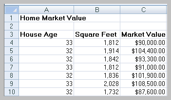
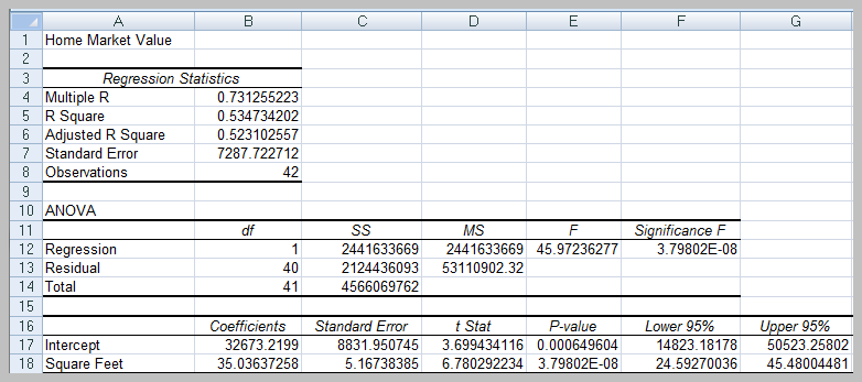
Example: Predicting home market value based on square footage.

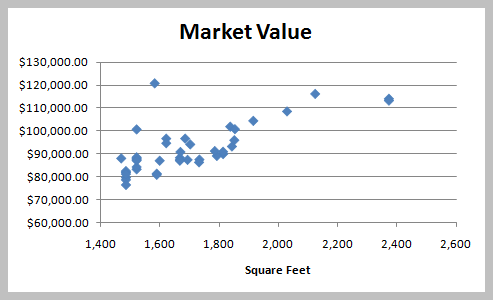
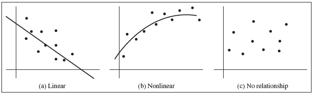
Assessing Linearity

Scatterplots help visualize the relationship between variables. The relationship can be linear, nonlinear, or show no relationship.

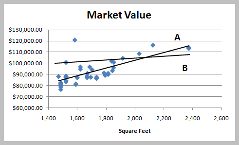
Fitting the Regression Line

Multiple lines can be drawn through the data, but the best fit is determined by minimizing the sum of squared residuals (least squares method).

Least Squares Regression

The least squares method estimates the regression coefficients by minimizing the sum of squared differences between observed and predicted values (residuals).

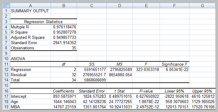
Interpreting Regression Output

Regression analysis output includes several key statistics:

• Multiple R: Correlation coefficient between observed and predicted values.

• R Square (R2): Proportion of variance in the dependent variable explained by the model (ranges from 0 to 1).

• Adjusted R Square: Adjusts R2 for the number of predictors and sample size.

• Standard Error: Standard deviation of the residuals.

• ANOVA Table: Tests overall model significance using the F-test.

• Coefficients: Estimates for intercept and slopes, with standard errors, t-statistics, and p-values for hypothesis testing.

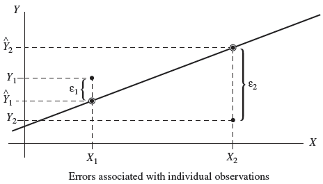
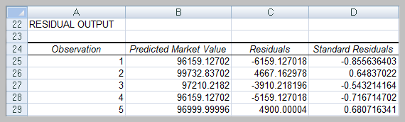
Residual Analysis

Residuals are the differences between observed and predicted values. Standardized residuals are used to assess model fit and check assumptions.

Assumptions of Regression

• Linearity: Relationship between X and Y is linear.

• Normality of Errors: Residuals are normally distributed with mean 0.

• Homoscedasticity: Constant variance of residuals across all levels of X.

• Independence: Residuals are independent.

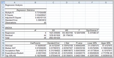
Multiple Linear Regression

Multiple regression extends simple regression to include multiple independent variables:

$Y = \beta_0 + \beta_1 X_1 + \beta_2 X_2 + ... + \beta_k X_k + \varepsilon$

Interpretation and model building involve checking the significance of each variable, using adjusted R2 for model comparison, and ensuring parsimony (simplicity).

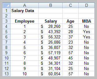
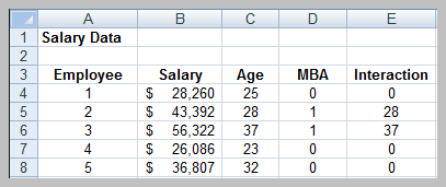
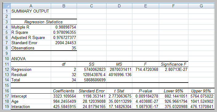
Regression with Categorical Variables and Interactions

Categorical variables are included using indicator (dummy) variables. Interaction terms allow the effect of one variable to depend on another.

Probability and Probability Distributions

Probability Concepts

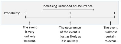
Probability quantifies the likelihood of an event occurring, ranging from 0 (impossible) to 1 (certain).

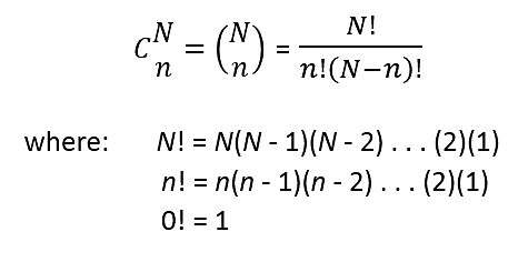
Counting Rules

• Combinations: Number of ways to choose n objects from N without regard to order.

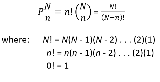
• Permutations: Number of ways to arrange n objects from N with regard to order.

Assigning Probabilities

• Classical Method: Assumes equally likely outcomes.

• Relative Frequency Method: Based on historical data.

• Subjective Method: Based on judgment or expert opinion.

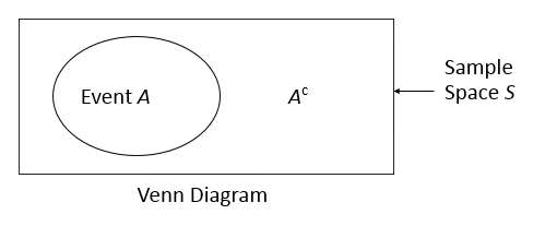
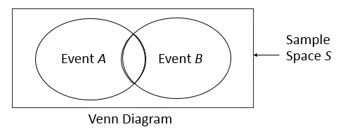
Events and Their Probabilities

• Event: A collection of sample points.

• Complement: All outcomes not in the event.

• Union: Outcomes in either of two events.

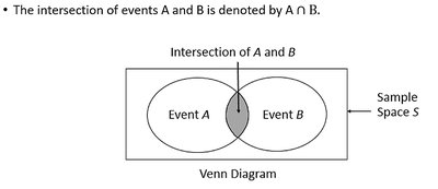
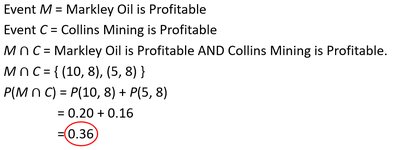
• Intersection: Outcomes in both events.

• Mutually Exclusive: Events that cannot occur together.

Conditional Probability and Independence

• Conditional Probability: Probability of A given B has occurred: $P(A|B) = \frac{P(A \cap B)}{P(B)}$

• Multiplication Law: $P(A \cap B) = P(A|B)P(B)$

• Independence: Events A and B are independent if $P(A|B) = P(A)$

Discrete Probability Distributions

Random Variables

A random variable assigns a numerical value to each outcome of an experiment. It can be discrete (countable values) or continuous (any value in an interval).

Discrete Probability Distribution

Describes the probability for each value of a discrete random variable. Must satisfy:

• All probabilities are between 0 and 1.

• The sum of all probabilities is 1.

Binomial Distribution

Models the number of successes in n independent trials, each with probability p of success.

$f(x) = \frac{n!}{x!(n-x)!} p^x (1-p)^{n-x}$

• Mean: $\mu = np$

• Variance: $\sigma^2 = np(1-p)$

• Standard Deviation: $\sigma = \sqrt{np(1-p)}$

Poisson Distribution

Models the number of occurrences in a fixed interval of time or space, given the average rate μ.

$f(x) = \frac{\mu^x e^{-\mu}}{x!}$

• Mean and Variance: Both equal to μ.

Continuous Probability Distributions

Uniform Distribution

All intervals of the same length are equally probable. The probability density function is:

$f(x) = \frac{1}{b-a}$ for $a \leq x \leq b$

• Mean: $E(x) = \frac{a+b}{2}$

• Variance: $Var(x) = \frac{(b-a)^2}{12}$

Normal Distribution

The normal distribution is symmetric and bell-shaped, defined by mean μ and standard deviation σ. The probability density function is:

$f(x) = \frac{1}{\sigma \sqrt{2\pi}} e^{-\frac{1}{2} \left(\frac{x-\mu}{\sigma}\right)^2}$

• 68.26% of values within ±1σ, 95.44% within ±2σ, 99.72% within ±3σ (Empirical Rule).

Standard Normal Distribution

A normal distribution with μ = 0 and σ = 1. Any normal variable can be converted to standard normal using:

$z = \frac{x-\mu}{\sigma}$

Exponential Distribution

Describes the time between events in a Poisson process. The probability density function is:

$f(x) = \frac{1}{\mu} e^{-x/\mu}$ for $x \geq 0$

• Mean and Standard Deviation: Both equal to μ.

Additional info: These notes cover the core concepts of regression analysis, probability, and probability distributions, with examples and outputs relevant to business statistics. All included images directly support the explanations provided.