Continuous Probability Distributions: Normal, Exponential, and Uniform Distributions

Chapter 6: Continuous Probability Distributions

6.1 Continuous Random Variables

Continuous random variables are variables that can take any value within a specified interval. They are distinguished from discrete random variables, which can only take specific, separate values. The probability of a continuous random variable taking any exact value is always zero; instead, probabilities are assigned to intervals of values.

• Definition: A continuous random variable is a variable whose possible values form an interval of numbers.

• Measurement Precision: The value depends on the precision of measurement (e.g., time to the nearest second, millisecond, etc.).

• Probability: Probability is determined for intervals, not specific values.

6.2 Continuous Probability Distributions

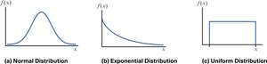
Continuous probability distributions describe the likelihood of all possible values of a continuous random variable. The three most common types are the normal, exponential, and uniform distributions.

• Normal Distribution: Data tend to cluster around a central value, with rare occurrences of extreme values.

• Exponential Distribution: Lower values are more common, and higher values are rare.

• Uniform Distribution: All values within a certain interval are equally likely.

6.2.1 Normal Probability Distributions

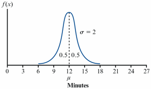
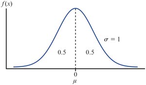
The normal distribution is a bell-shaped, symmetrical distribution centered around the mean. It is widely used in statistics due to its natural occurrence in many real-world phenomena.

• Symmetry: The distribution is symmetric about the mean (μ), so the mean and median are equal.

• Probability Density Function (PDF): The total area under the curve is 1.0, with 0.5 to the left and right of the mean.

• Tails: The curve extends indefinitely in both directions, never touching the horizontal axis.

Parameters of the Normal Distribution

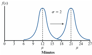
• Mean (μ): Determines the center of the distribution.

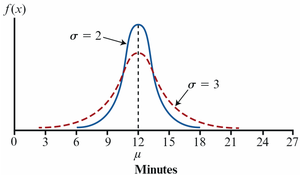
• Standard Deviation (σ): Determines the spread or width of the distribution.

• Effect of Changing Parameters: Changing μ shifts the curve left or right; changing σ stretches or compresses the curve.

Normal Probability Density Function (PDF)

The mathematical formula for the normal PDF is:

$f(x) = \frac{1}{\sigma \sqrt{2\pi}} e^{-(1/2)[(x-\mu)/\sigma]^2}$

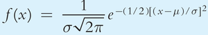
• e: Euler's number, approximately 2.71828

• π: Pi, approximately 3.14159

• μ: Mean of the distribution

• σ: Standard deviation of the distribution

• x: Value of interest

Standard Normal Distribution and z-Scores

The standard normal distribution is a special case with μ = 0 and σ = 1. Any normal distribution can be converted to the standard normal using the z-score formula:

$z = \frac{x - \mu}{\sigma}$

• z-Score: Indicates how many standard deviations a value x is from the mean.

• Negative z: x is below the mean.

• Positive z: x is above the mean.

• At the mean: z = 0.

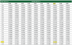
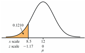
Calculating Probabilities Using z-Scores

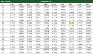
To find probabilities, convert x to a z-score and use the standard normal table (z-table) to find the area under the curve.

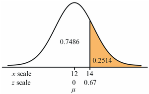
• Example: Mean call time μ = 12 min, σ = 3 min. Probability that a call lasts 14 min or less?

$z_{14} = \frac{14 - 12}{3} = 0.67$

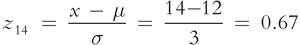
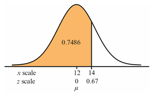
• From the z-table, P(z ≤ 0.67) ≈ 0.7486

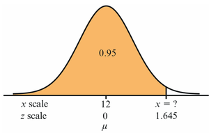
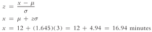
Finding x for a Given Probability

• To find the value x corresponding to a cumulative probability (e.g., 95%), use the z-score for that probability and solve for x:

$x = \mu + z\sigma$

Negative z-Scores

• For values below the mean, z is negative. Use the z-table for negative values to find probabilities.

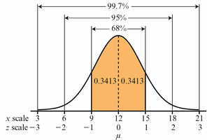
The Empirical Rule

The empirical rule states that for a normal distribution:

• 68% of values fall within 1 standard deviation of the mean

• 95% within 2 standard deviations

• 99.7% within 3 standard deviations

Probability Intervals: Real-World Example

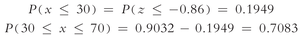
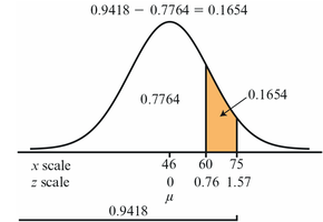
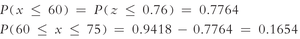
Suppose annual snowfall in Minneapolis is normally distributed with μ = 46 in., σ = 18.5 in. What is the probability that snowfall is between 30 and 70 inches?

• Calculate z-scores for x = 30 and x = 70:

$z_{30} = \frac{30 - 46}{18.5} = -0.86$ $z_{70} = \frac{70 - 46}{18.5} = 1.30$

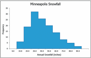
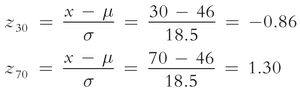
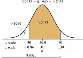
From the z-table:

$P(x \leq 30) = 0.1949$ $P(x \leq 70) = 0.9032$ $P(30 \leq x \leq 70) = 0.9032 - 0.1949 = 0.7083$

Other Probability Intervals

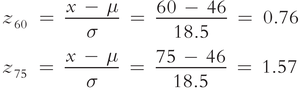
• Probability between 60 and 75 inches: Calculate z-scores, find areas, and subtract as above.

$P(60 \leq x \leq 75) = 0.9418 - 0.7764 = 0.1654$

Excel Functions for Normal Probabilities

• NORM.DIST(x, mean, standard_dev, cumulative): Returns the cumulative probability for a normal distribution.

• NORM.S.DIST(z, cumulative): Returns the cumulative probability for the standard normal distribution.

6.2.2 Using the Normal Distribution to Approximate the Binomial Distribution

When the sample size is large and both np ≥ 5 and nq ≥ 5, the normal distribution can approximate the binomial distribution. A continuity correction (±0.5) is applied when converting discrete x values to the continuous normal scale.

• Application: Used in quality control and other business contexts.

• Continuity Correction: Add or subtract 0.5 to x when using the normal approximation.

6.3 Exponential Probability Distributions

The exponential distribution models the time between events in a process where events occur continuously and independently at a constant average rate.

• Right-Skewed: Most values are near zero, with a long tail to the right.

• Parameter: Defined by λ (rate of occurrence).

• PDF: $f(x) = \lambda e^{-\lambda x}$ for x ≥ 0

• Mean: $\mu = 1/\lambda$

• Standard Deviation: $\sigma = 1/\lambda$

6.4 Uniform Probability Distributions

In a continuous uniform distribution, all intervals of the same length within the distribution's range are equally probable.

• PDF: $f(x) = \frac{1}{b - a}$ for $a \leq x \leq b$

• CDF: $F(x) = \frac{x - a}{b - a}$ for $a \leq x \leq b$

• Mean: $\mu = \frac{a + b}{2}$

• Standard Deviation: $\sigma = \frac{b - a}{\sqrt{12}}$

Example: Exam Completion Time

If exam times are uniformly distributed between 70 and 120 minutes, the probability that a student finishes in less than 80 minutes is:

$P(x \leq 80) = \frac{80 - 70}{120 - 70} = \frac{10}{50} = 0.2$

Summary Table: Key Properties of Continuous Distributions

Distribution	Shape	Parameters	PDF	Mean	Standard Deviation
Normal	Bell-shaped, symmetric	μ, σ	$f(x) = \frac{1}{\sigma \sqrt{2\pi}} e^{-(1/2)[(x-\mu)/\sigma]^2}$	μ	σ
Exponential	Right-skewed	λ	$f(x) = \lambda e^{-\lambda x}$	$1/\lambda$	$1/\lambda$
Uniform	Rectangular	a, b	$f(x) = \frac{1}{b - a}$	$\frac{a + b}{2}$	$\frac{b - a}{\sqrt{12}}$