Continuous Probability Distributions: Normal, Exponential, and Uniform Distributions

Continuous Probability Distributions

Overview of Continuous Probability Distributions

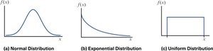
Continuous probability distributions describe the probabilities of the possible values of a continuous random variable. The three most common types are the Normal, Exponential, and Uniform distributions. Each has distinct characteristics and applications in business statistics.

• Normal Distribution: Bell-shaped and symmetric, commonly used for naturally occurring data.

• Exponential Distribution: Right-skewed, used for modeling time between events.

• Uniform Distribution: All intervals of the same width are equally probable.

Continuous Random Variables

Definition and Properties

A continuous random variable can take any value within a given interval. The probability of the variable taking any exact value is zero; instead, probabilities are assigned to intervals. The precision of measurement affects the value observed.

Normal Probability Distributions

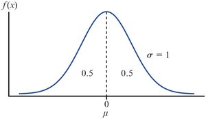
Characteristics of the Normal Distribution

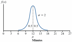
The normal probability distribution is bell-shaped and symmetric about the mean. It is widely used because many natural phenomena approximate this distribution. The mean (μ) and standard deviation (σ) fully describe its shape.

• The mean, median, and mode are equal.

• The total area under the curve is 1.0.

• The distribution extends indefinitely in both directions.

• Values near the mean are most probable.

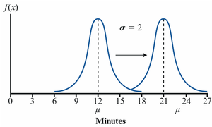
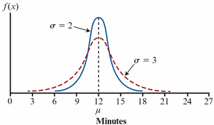
Effect of Mean and Standard Deviation

Changing the mean (μ) shifts the distribution left or right, while changing the standard deviation (σ) alters the spread of the curve.

Normal Probability Density Function

The mathematical expression for the normal probability density function is:

$f(x) = \frac{1}{\sigma \sqrt{2\pi}} e^{-(1/2)[(x-\mu)/\sigma]^2}$

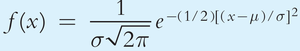
where: $\mu$ = mean $\sigma$ = standard deviation $x$ = value of interest $e \approx 2.71828$, $\pi \approx 3.14159$

The Standard Normal Distribution and z-Scores

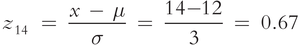
The standard normal distribution is a special case with $\mu = 0$ and $\sigma = 1$. Any normal distribution can be converted to the standard normal using the z-score:

$z = \frac{x - \mu}{\sigma}$

• z-scores indicate how many standard deviations a value is from the mean.

• Negative z-scores are below the mean; positive are above.

Calculating Probabilities Using z-Scores

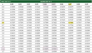
To find the probability that a value falls below a certain point, calculate its z-score and use the standard normal table.

Example: For $x = 14$, $\mu = 12$, $\sigma = 3$:

$z_{14} = \frac{14 - 12}{3} = 0.67$

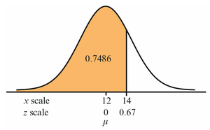
From the normal table, $P(x \leq 14) = 0.7486$.

Finding Probabilities for Intervals

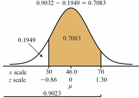
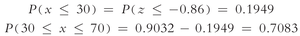
To find the probability that a value falls between two points, calculate the z-scores for both endpoints and subtract the smaller cumulative probability from the larger.

Example: Probability between $x = 30$ and $x = 70$ for $\mu = 46$, $\sigma = 18.5$:

$z_{30} = \frac{30 - 46}{18.5} = -0.86$ $z_{70} = \frac{70 - 46}{18.5} = 1.30$

$P(30 \leq x \leq 70) = P(z \leq 1.30) - P(z \leq -0.86) = 0.9032 - 0.1949 = 0.7083$

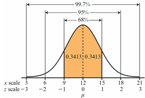
The Empirical Rule

The empirical rule states that for a normal distribution:

• 68% of values fall within 1 standard deviation of the mean

• 95% within 2 standard deviations

• 99.7% within 3 standard deviations

Using Excel for Normal Probabilities

Excel functions for normal probabilities:

• NORM.DIST(x, mean, standard_dev, cumulative): Returns the cumulative probability for a normal distribution.

• NORM.S.DIST(z, cumulative): Returns the cumulative probability for the standard normal distribution.

Exponential Probability Distributions

Definition and Applications

The exponential probability distribution models the time between events in a process where events occur continuously and independently at a constant average rate. It is right-skewed and described by the parameter $\lambda$ (rate).

• Common applications: time between customer arrivals, time until equipment failure.

Probability Density Function

The exponential probability density function is:

$f(x) = \lambda e^{-\lambda x}$, for $x \geq 0$

where $\lambda$ is the rate parameter (mean number of occurrences per interval).

Cumulative Distribution Function

The cumulative distribution function (CDF) is:

$F(a) = 1 - e^{-\lambda a}$

Relationship to Poisson Distribution

If the number of events in an interval follows a Poisson distribution with mean $\lambda$, the time between events follows an exponential distribution with mean $\mu = 1/\lambda$.

Excel for Exponential Probabilities

Excel function: EXPON.DIST(x, lambda, cumulative)

• Set cumulative = TRUE for the cumulative probability.

Uniform Probability Distributions

Definition and Properties

The continuous uniform probability distribution assigns equal probability to all intervals of the same width within a specified range [a, b].

• Probability density function: $f(x) = \frac{1}{b - a}$ for $a \leq x \leq b$

• Cumulative distribution function: $F(x) = \frac{x - a}{b - a}$ for $a \leq x \leq b$

Mean and Standard Deviation

The mean and standard deviation for the uniform distribution are:

Mean: $\mu = \frac{a + b}{2}$ Standard deviation: $\sigma = \frac{b - a}{\sqrt{12}}$

Example Application

Suppose the time to finish a statistics exam is uniformly distributed between 70 and 120 minutes. The probability that a student finishes in less than 80 minutes is:

$P(x \leq 80) = \frac{80 - 70}{120 - 70} = \frac{10}{50} = 0.2$

Summary Table: Key Properties of Continuous Distributions

Distribution	Shape	Parameters	Typical Application
Normal	Bell-shaped, symmetric	Mean (μ), Std. Dev. (σ)	Heights, test scores, measurement errors
Exponential	Right-skewed	Rate (λ)	Time between arrivals, lifetimes
Uniform	Rectangular	Min (a), Max (b)	Random number generation, waiting times