Continuous Probability Distributions: The Normal Distribution and Its Applications

Continuous Probability Distributions

Introduction to Continuous Probability Distributions

Continuous probability distributions describe the probabilities of the possible values of a continuous random variable. Unlike discrete random variables, which take on countable values, continuous random variables can assume any value within a given interval. Examples include measurements such as time, distance, and weight.

• Continuous random variables are usually measured, not counted.

• Probabilities are assigned to intervals, not individual values.

• The probability of any single, exact value is theoretically zero; probability is represented by the area under the curve of the distribution.

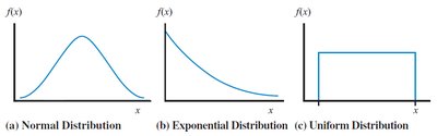
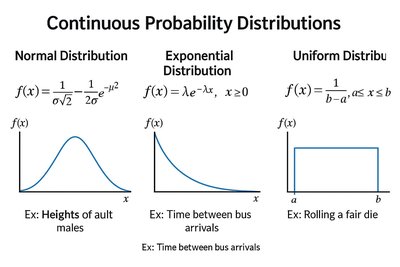
Types of Continuous Probability Distributions

The three most common continuous probability distributions are the normal, exponential, and uniform distributions. Each has distinct characteristics and applications in business statistics.

• Normal Distribution: Bell-shaped, symmetrical, and describes many natural phenomena.

• Exponential Distribution: Describes the time between events in a Poisson process; lower values are more common.

• Uniform Distribution: All outcomes in the interval are equally likely.

The Normal Probability Distribution

Characteristics of the Normal Distribution

The normal distribution is one of the most important probability distributions in statistics. It is used extensively in business for modeling variables that tend to cluster around a mean.

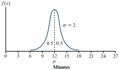
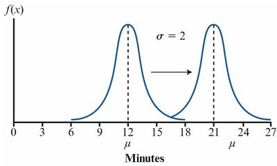
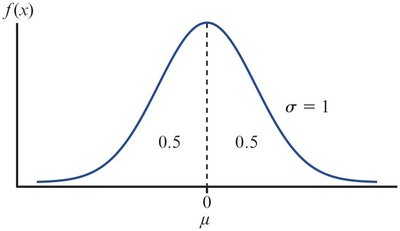
• The distribution is bell-shaped and symmetrical around the mean (μ).

• The mean, median, and mode are all equal.

• The total area under the curve is 1.0, with 0.5 to the left and 0.5 to the right of the mean.

• The curve extends indefinitely in both directions, never touching the horizontal axis.

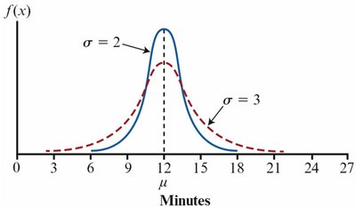
• The shape is completely described by its mean (μ) and standard deviation (σ).

The Normal Probability Density Function

The probability density function (PDF) for the normal distribution is given by:

$f(x) = \frac{1}{\sigma \sqrt{2\pi}} e^{-\frac{1}{2} \left( \frac{x-\mu}{\sigma} \right)^2}$

• Where μ is the mean, σ is the standard deviation, and x is the value of interest.

• The PDF describes the relative likelihood for the random variable to take on a given value.

Standard Normal Distribution and z-Scores

Any normal distribution can be transformed into the standard normal distribution, which has a mean of 0 and a standard deviation of 1. This transformation uses the z-score formula:

$z = \frac{x - \mu}{\sigma}$

• A z-score indicates how many standard deviations a value is from the mean.

• z-scores are negative for values below the mean and positive for values above the mean.

• The standard normal distribution is used to find probabilities using normal probability tables.

Using Normal Probability Tables

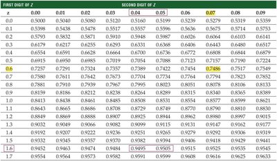
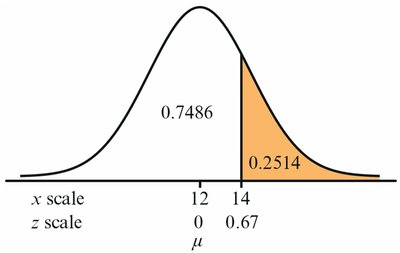
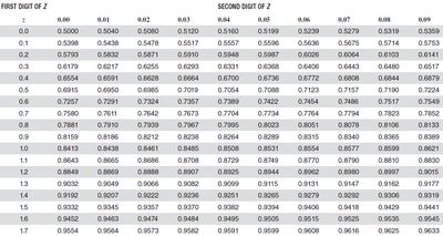
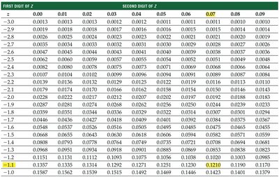
Normal probability tables (z-tables) provide the cumulative area under the standard normal curve to the left of a given z-score. To find probabilities for a normal distribution:

1. Convert the value of interest (x) to a z-score using the formula above.

2. Look up the z-score in the normal probability table to find the corresponding probability.

3. For upper-tail probabilities, subtract the table value from 1.

Empirical Rule (68-95-99.7 Rule)

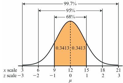
The empirical rule states that for a normal distribution:

• Approximately 68% of values fall within one standard deviation of the mean (μ ± 1σ).

• Approximately 95% fall within two standard deviations (μ ± 2σ).

• Approximately 99.7% fall within three standard deviations (μ ± 3σ).

Examples and Applications

Normal distributions are used in a variety of business contexts, such as modeling customer wait times, inventory demand, and quality control. Below are several worked examples:

Example: Probability Between Two Values

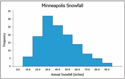
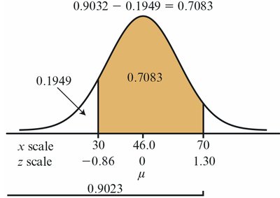
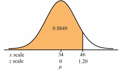
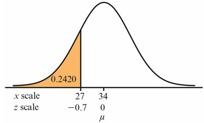
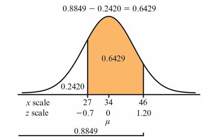
• Suppose annual snowfall in Minneapolis is normally distributed with μ = 46 inches and σ = 18.5 inches. What is the probability that between 30 and 70 inches of snow will fall next year?

• Calculate z-scores for x = 30 and x = 70:

• Find probabilities using the z-table and subtract to get the probability for the interval:

Example: Probability for an Upper Interval

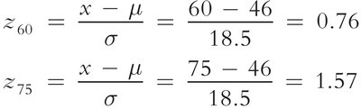
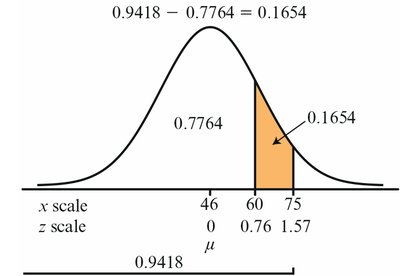
• What is the probability that between 60 and 75 inches of snow will fall?

• Calculate z-scores for x = 60 and x = 75:

• Find probabilities and subtract:

Example: Probability for a Lower Interval

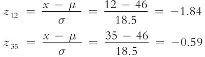
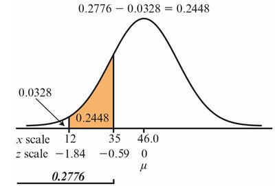
• What is the probability that between 12 and 35 inches of snow will fall?

• Calculate z-scores for x = 12 and x = 35:

• Find probabilities and subtract:

Calculating Normal Probabilities Using Excel

Excel provides built-in functions for calculating normal probabilities:

• NORM.DIST(x, mean, standard_dev, cumulative): Returns the probability for a normal distribution. Set cumulative = TRUE for cumulative probability.

• NORM.S.DIST(z, cumulative): Returns the probability for the standard normal distribution.

Using the Normal Distribution to Approximate the Binomial Distribution

Normal Approximation to the Binomial

When the sample size is large and both np ≥ 5 and nq ≥ 5, the normal distribution can be used to approximate the binomial distribution. This is useful because normal probabilities are easier to calculate than binomial probabilities for large n.

• Mean: $\mu = np$

• Standard deviation: $\sigma = \sqrt{npq}$

• Apply a continuity correction by adjusting the interval by 0.5 units when approximating discrete probabilities.

Example: Quality Control Application

• Suppose a fast-food chain has a 6% error rate in orders. For 120 orders, what is the probability that exactly 7 will have errors?

• Calculate mean and standard deviation, then use the normal approximation with continuity correction (6.5 to 7.5):

Summary Table: Key Properties of the Normal Distribution

Property	Description
Shape	Bell-shaped, symmetrical
Parameters	Mean (μ), Standard Deviation (σ)
Total Area	1.0
Empirical Rule	68% within 1σ, 95% within 2σ, 99.7% within 3σ
Standard Normal	μ = 0, σ = 1

Additional info: The notes above include expanded academic context, formulas, and examples to ensure completeness and clarity for exam preparation in a Statistics for Business course.