Correlation and Simple Linear Regression: Chapter 14 Study Guide

Correlation and Simple Linear Regression

14.1 Dependent and Independent Variables

In regression and correlation analysis, variables are classified as either independent or dependent. The independent variable (x) is used to explain or predict the dependent variable (y). The direction of causality is assumed to be from x to y.

• Independent Variable (x): The variable that is manipulated or used as a predictor.

• Dependent Variable (y): The variable that is measured or predicted.

• Examples: The size of a television screen (x) explains the selling price (y); the number of visitors per day (x) explains the amount of sales per day (y).

Independent Variable	Dependent Variable
The size of a television screen	The selling price of the television
The number of visitors per day on a Web site	The amount of sales per day from the Web site
The curb weight of a car	The car's gas mileage

14.2 Correlation Analysis

Correlation analysis measures the strength and direction of a linear relationship between two variables. A relationship is linear if the scatter plot of the variables forms a straight-line pattern.

• Strength: How closely the data points fit a straight line.

• Direction: Positive (both variables increase together) or negative (one increases as the other decreases).

• Scatter Plot: Used to visually assess linearity.

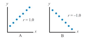
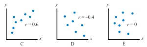
Correlation Coefficient (r): Indicates both strength and direction. Values range from -1.0 (perfect negative) to +1.0 (perfect positive). r = 0 means no linear relationship.

• Perfect Positive: $r = 1.0$

• Perfect Negative: $r = -1.0$

• Moderate Positive: $r = 0.6$

• Moderate Negative: $r = -0.4$

• No Correlation: $r = 0$

Formula for the Correlation Coefficient:

$r = \frac{n\sum xy - \sum x \sum y}{\sqrt{[n\sum x^2 - (\sum x)^2][n\sum y^2 - (\sum y)^2]}}$

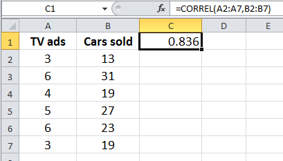
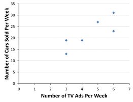
Example: Using Excel's CORREL function to calculate r for TV ads and cars sold.

Hypothesis Testing for the Correlation Coefficient

To determine if the population correlation coefficient ($\rho$) is significantly different from zero, a hypothesis test is performed:

• Null Hypothesis (H0): $\rho \leq 0$ (no positive relationship)

• Alternative Hypothesis (H1): $\rho > 0$ (positive linear relationship)

Test Statistic:

$t = \frac{r\sqrt{n-2}}{\sqrt{1-r^2}}$

Compare t to the critical value from the t-distribution with $n-2$ degrees of freedom.

14.3 Simple Linear Regression Analysis

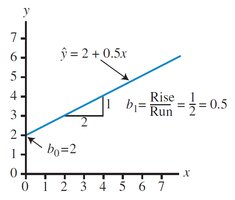
Simple linear regression fits a straight line to a set of ordered pairs (x, y) to model the relationship between the independent and dependent variables. The regression equation is:

$\hat{y} = b_0 + b_1x$

• $\hat{y}$: Predicted value of y

• $b_0$: y-intercept

• $b_1$: Slope

Residuals (ei): The difference between the actual and predicted values for each observation.

$e_i = y_i - \hat{y}_i$

Least Squares Method: Minimizes the sum of squared errors (SSE) to find the best fit line.

$SSE = \sum (y_i - \hat{y}_i)^2$

Formulas for Slope and Intercept:

$b_1 = \frac{\sum (x_i - \bar{x})(y_i - \bar{y})}{\sum (x_i - \bar{x})^2}$

$b_0 = \bar{y} - b_1\bar{x}$

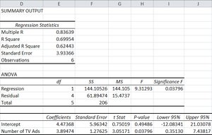
Example: Regression equation for TV ads and cars sold.

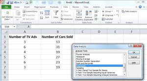
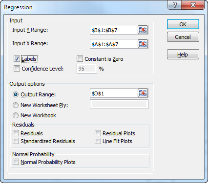
Calculating Regression in Excel

Excel's Data Analysis tool can be used to perform regression analysis. Input the dependent and independent variables, select regression, and review the output for coefficients, standard error, and significance.

Partitioning the Sum of Squares

The total variation in the dependent variable is partitioned into explained and unexplained components:

• Total Sum of Squares (SST): $SST = \sum (y_i - \bar{y})^2$

• Sum of Squares Regression (SSR): $SSR = \sum (\hat{y}_i - \bar{y})^2$

• Sum of Squares Error (SSE): $SSE = \sum (y_i - \hat{y}_i)^2$

• Relationship: $SST = SSR + SSE$

Coefficient of Determination (R2)

R2 measures the proportion of variation in y explained by x. It ranges from 0 to 1 (or 0% to 100%).

$R^2 = \frac{SSR}{SST}$

Higher values indicate a better fit.

Hypothesis Testing for R2

To test if the population coefficient of determination ($\rho^2$) is significantly greater than zero:

• Null Hypothesis (H0): $\rho^2 \leq 0$

• Alternative Hypothesis (H1): $\rho^2 > 0$

F-test Statistic:

$F = \frac{SSR / 1}{SSE / (n-2)}$

14.4 Using Regression to Make Predictions

Regression equations can be used to predict y for a given x. A point estimate is the predicted value, and confidence intervals can be constructed around this estimate.

• Standard Error of Estimate (se): Measures dispersion of observed data around the regression line.

Confidence Interval for Average y:

$CI = \hat{y} \pm t_{\alpha/2} \cdot se \cdot \sqrt{\frac{1}{n} + \frac{(x_i - \bar{x})^2}{\sum (x_j - \bar{x})^2}}$

Prediction Interval for Specific y:

$PI = \hat{y} \pm t_{\alpha/2} \cdot se \cdot \sqrt{1 + \frac{1}{n} + \frac{(x_i - \bar{x})^2}{\sum (x_j - \bar{x})^2}}$

14.5 Testing the Significance of the Slope

To determine if the slope ($b_1$) is significantly different from zero, a t-test is performed:

• Null Hypothesis (H0): $\beta_1 = 0$

• Alternative Hypothesis (H1): $\beta_1 \neq 0$

Test Statistic:

$t = \frac{b_1 - \beta_1}{s_b}$

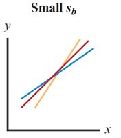
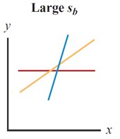
Standard Error of Slope (sb): Measures variation in the estimate of the slope.

14.6 Assumptions for Regression Analysis

Regression analysis relies on several key assumptions:

• Linearity: The relationship between x and y is linear.

• Independence: Residuals are independent and exhibit no patterns.

• Homoscedasticity: Constant variance of residuals across values of x.

• Normality: Residuals follow a normal distribution.

Scatter plots and residual plots are used to check these assumptions.

14.7 Simple Regression Example with Negative Correlation

Regression can also model negative relationships. For example, as driving speed increases, gas mileage decreases. The slope of the regression equation is negative.

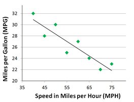
Example: For each 1 MPH increase in speed, gas mileage decreases by 0.26 MPG.

14.8 Final Thoughts and Pitfalls

Key cautions in regression analysis:

• Do not extrapolate: Avoid predicting y for x values outside the observed range.

• Correlation does not imply causation: Statistical significance does not prove causality.

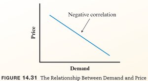
Example: The law of supply and demand demonstrates negative correlation: as price increases, demand decreases.

Summary: Correlation and regression are powerful tools for analyzing relationships between variables, but must be used with care and proper understanding of their assumptions and limitations.