Correlation and Simple Linear Regression: Concepts, Calculations, and Applications

Correlation and Simple Linear Regression

14.1 Dependent and Independent Variables

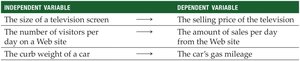
In statistical modeling, variables are classified as either independent (explanatory) or dependent (response). The independent variable, denoted as x, is used to explain or predict changes in the dependent variable, y. The direction of explanation is one-way: changes in x are used to explain changes in y, not vice versa.

• Independent Variable (x): The variable that is manipulated or categorized to observe its effect on the dependent variable.

• Dependent Variable (y): The outcome or variable being predicted or explained.

Examples:

Independent Variable	Dependent Variable
The size of a television screen	The selling price of the television
The number of visitors per day on a website	The amount of sales per day from the website
The curb weight of a car	The car's gas mileage

14.2 Correlation Analysis

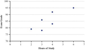
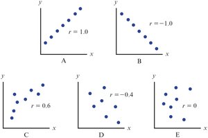
Correlation analysis measures the strength and direction of a linear relationship between two variables. A relationship is considered linear if a scatter plot of the variables forms a straight-line pattern.

• Strength: How closely the data points fit a straight line.

• Direction: Positive (both variables increase together) or negative (one increases as the other decreases).

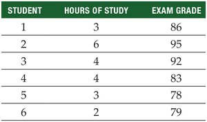
Example: Investigating the relationship between hours studied and exam grades for six students.

Student	Hours of Study	Exam Grade
1	3	86
2	6	95
3	4	92
4	4	83
5	3	78
6	2	79

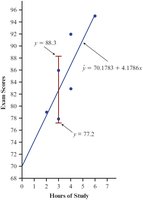
The scatter plot visually displays the relationship:

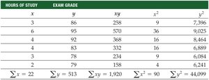
Summary Table for Calculations

To compute correlation and regression, a summary table of calculations is constructed:

Sample Correlation Coefficient (r)

The correlation coefficient (r) quantifies the strength and direction of the linear relationship. Its value ranges from -1 (perfect negative) to +1 (perfect positive). r = 0 indicates no linear relationship.

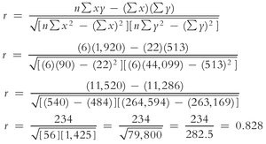
The formula for the sample correlation coefficient is:

$r = \frac{n\sum xy - (\sum x)(\sum y)}{\sqrt{[n\sum x^2 - (\sum x)^2][n\sum y^2 - (\sum y)^2]}}$

Substituting the values from the example:

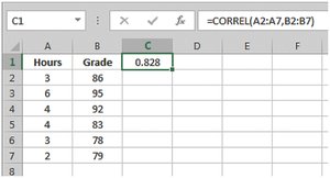
Using Excel: The correlation coefficient can be calculated using =CORREL(array1, array2).

Hypothesis Test for Correlation Coefficient

To determine if the population correlation coefficient (ρ) is significantly different from zero, a hypothesis test is conducted:

• Null hypothesis: $H_0: \rho \leq 0$

• Alternative hypothesis: $H_1: \rho > 0$

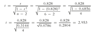
The test statistic is:

$t = \frac{r}{\sqrt{\frac{1 - r^2}{n - 2}}}$

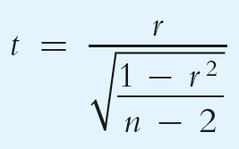
Example calculation:

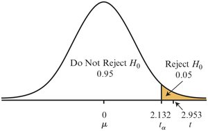
Critical values are compared to determine significance. If the calculated t is greater than the critical value, the null hypothesis is rejected.

14.3 Simple Linear Regression Analysis

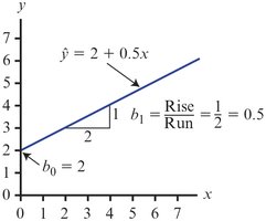
Simple linear regression describes the best-fitting straight line through a set of (x, y) pairs, using only one independent variable. The regression equation is:

$\hat{y} = b_0 + b_1 x$

• \( \hat{y} \): Predicted value of y

• \( b_0 \): y-intercept

• \( b_1 \): Slope

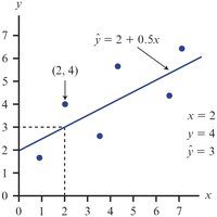
The difference between the actual and predicted values is called the residual:

$e_i = y_i - \hat{y}_i$

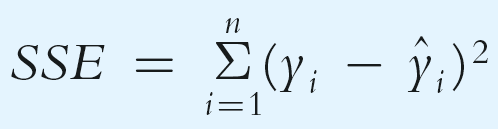
The Least Squares Method

The least squares method finds the regression line that minimizes the sum of squared errors (SSE):

$SSE = \sum_{i=1}^n (y_i - \hat{y}_i)^2$

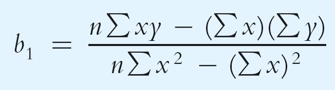
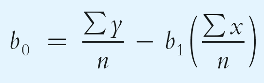
Calculating Slope and Intercept

The formulas for the regression slope and intercept are:

$b_1 = \frac{n\sum xy - (\sum x)(\sum y)}{n\sum x^2 - (\sum x)^2}$

$b_0 = \frac{\sum y}{n} - b_1 \left(\frac{\sum x}{n}\right)$

Example calculation for the exam data:

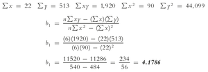
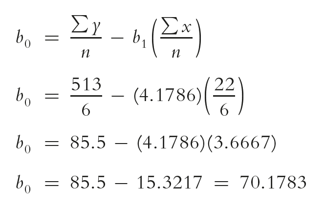
Interpretation: Each additional hour of study increases the predicted exam score by 4.18 points.

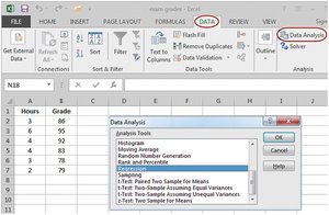
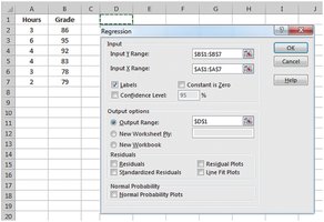
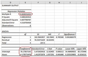
Using Excel for Regression

Excel's Data Analysis tool can be used to perform regression analysis, providing coefficients, R-squared, and other statistics.

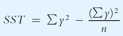
Partitioning the Sum of Squares

The total sum of squares (SST) measures the total variation in the dependent variable. It is partitioned into:

• SSR (Regression Sum of Squares): Variation explained by the regression

• SSE (Error Sum of Squares): Unexplained variation

$SST = \sum y^2 - \frac{(\sum y)^2}{n}$

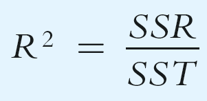
Coefficient of Determination (R2)

The coefficient of determination (R2) measures the proportion of total variation in the dependent variable explained by the independent variable:

$R^2 = \frac{SSR}{SST}$

Example calculation:

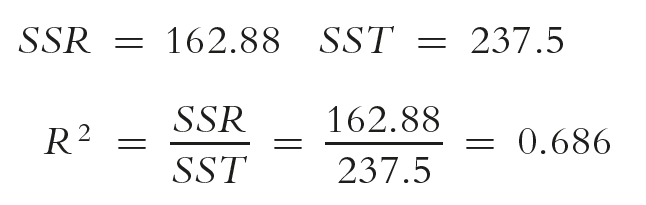
Interpretation: 68.6% of the variation in exam grades is explained by hours studied.

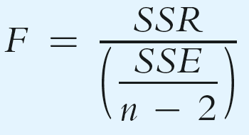
Hypothesis Test for R2

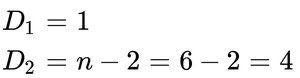
To test if the population coefficient of determination is significantly greater than zero, use the F-test:

$F = \frac{SSR}{\left(\frac{SSE}{n-2}\right)}$

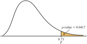
Example calculation:

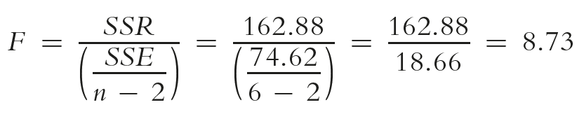
Compare the calculated F to the critical value. If F is greater, reject the null hypothesis.

The p-value can also be used for decision-making.

14.4 Using Regression to Make Predictions

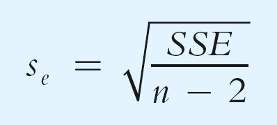
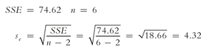
To predict the value of y for a given x, substitute x into the regression equation. A confidence interval can be constructed around the point estimate using the standard error of the estimate (se):

$s_e = \sqrt{\frac{SSE}{n-2}}$

Example calculation:

Confidence Interval for Average Value of y

The confidence interval for the average value of y at a given x is:

$CI = \hat{y} \pm t_{\alpha/2} s_e \sqrt{\frac{1}{n} + \frac{(x - \bar{x})^2}{\sum x^2 - \frac{(\sum x)^2}{n}}}$

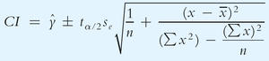
Example calculation:

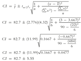
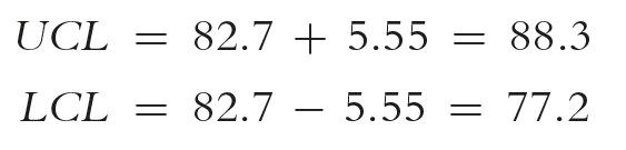
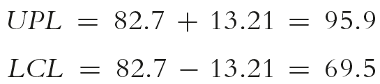
Upper and lower confidence limits:

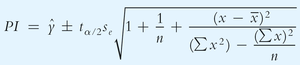
Prediction Interval for a Specific Value of y

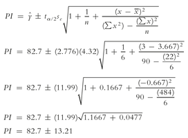
The prediction interval for an individual value of y at a given x is wider than the confidence interval for the mean:

$PI = \hat{y} \pm t_{\alpha/2} s_e \sqrt{1 + \frac{1}{n} + \frac{(x - \bar{x})^2}{\sum x^2 - \frac{(\sum x)^2}{n}}}$

Example calculation:

14.5 Testing the Significance of the Slope

To determine if the independent variable significantly predicts the dependent variable, test the null hypothesis that the population slope (β1) is zero:

• Null hypothesis: $H_0: \beta_1 = 0$

• Alternative hypothesis: $H_1: \beta_1 \neq 0$

The test statistic is:

$t = \frac{b_1 - \beta_1}{s_b}$

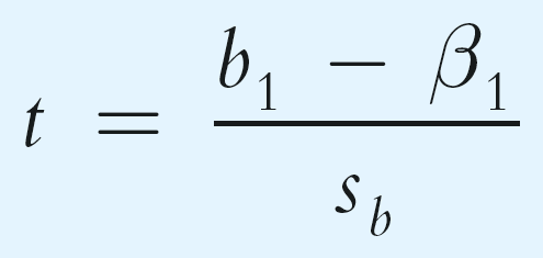
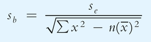
The standard error of the slope is:

$s_b = \frac{s_e}{\sqrt{\sum x^2 - n(\bar{x})^2}}$

Confidence Interval for the Slope

The confidence interval for the population slope is:

$b_1 \pm t_{\alpha/2} s_b$

Interpretation: If the interval does not include zero, there is evidence of a linear relationship.

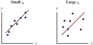
14.6 Assumptions for Regression Analysis

For regression results to be valid, several assumptions must be met:

• Linearity: The relationship between x and y is linear.

• Independence: Residuals are independent.

• Homoscedasticity: Constant variance of residuals across values of x.

• Normality: Residuals are normally distributed.

Scatter plots and residual plots are used to check these assumptions.

14.7 Simple Regression with Negative Correlation

When the slope of the regression line is negative, the variables have a negative linear relationship. For example, as the price of a product increases, demand typically decreases.

14.8 Final Thoughts

• Do not extrapolate: Avoid predicting values outside the observed range of x.

• Correlation is not causation: A significant relationship does not imply that x causes changes in y.