Exploratory Data Analysis I: One Parameter – Foundations of Business Statistics

Statistics, Data, and Statistical Thinking

Introduction to Data and Statistics

Statistics is the science of collecting, analyzing, interpreting, and presenting data to support decision-making. In business, data can come from surveys, transactions, time series, or digital sources such as social media and autonomous systems.

• Data: Observations gathered on characteristics of interest (e.g., survey responses, transaction records).

• Examples: Economic indicators, payment transactions, social media data, sensor data from vehicles.

Why Do We Need Statistics?

Statistics enables us to make sense of data, derive patterns, and support or refute theories. It is essential for making informed business decisions.

The PPDAC Cycle

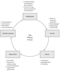
The PPDAC cycle is a structured approach to statistical inquiry, guiding the process from problem definition to conclusion.

• Problem: Define and understand the question.

• Plan: Decide what to measure, how, and design the study.

• Data: Collect, manage, and clean the data.

• Analysis: Sort, construct tables/graphs, and look for patterns.

• Conclusion: Interpret results, draw conclusions, and communicate findings.

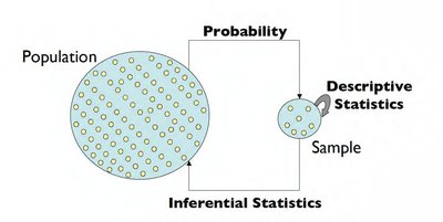
Descriptive and Inferential Statistics

Types of Statistical Analysis

There are two main branches of statistics:

• Descriptive Statistics (Exploratory Data Analysis): Summarizes and describes the main features of a dataset using summary statistics and graphical representations.

• Inferential Statistics: Makes predictions or inferences about a population based on sample data, using probability theory.

Key Statistical Terms

• Population: The entire set of subjects of interest.

• Parameter: A numerical summary of the population (e.g., population mean).

• Sample: A subset of the population used for analysis.

• Sample Statistic: A numerical summary of the sample data (e.g., sample mean).

Example: Airport Satisfaction Survey

• Population: All passengers’ satisfaction ratings (e.g., 30 million per year).

• Parameter: Mean satisfaction rating of all passengers.

• Sample: 2,000 respondents’ ratings.

• Sample Statistic: Mean rating of the 2,000 respondents.

Sources of Error in Inference

Inference involves uncertainty due to differences between the sample and the population. Probability theory and statistical methods (e.g., sampling distributions, confidence intervals, hypothesis testing) help quantify and manage this uncertainty.

Tabular and Graphical Presentation of Data

Data Types

Understanding data types is crucial for choosing appropriate summary and visualization methods.

• Quantitative Data: Numerical values (can be continuous or discrete).

• Qualitative Data: Non-numerical, categorical values (can be nominal or ordinal).

• Continuous: Infinite possible values (e.g., height, commuting time).

• Discrete: Finite number of values (e.g., number of siblings, letter grades).

• Ordinal: Categories with a natural order (e.g., cell size level, letter grades).

• Nominal: Categories without a natural order (e.g., favorite colors, college major).

Summarizing Qualitative-Nominal Data

Frequency distributions and bar plots are commonly used to summarize categorical data.

Soft Drink	Frequency	Proportion	Percentage
Coca-Cola	19	0.38	38
Diet Coke	8	0.16	16
Dr. Pepper	5	0.10	10
Pepsi	13	0.26	26
Sprite	5	0.10	10
Total	50	1.00	100

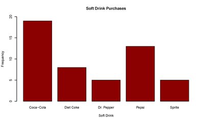
Good and Bad Graphs

A good graph is clear, matches the data type, and includes informative titles, labels, and scales. Avoid unnecessary complexity (e.g., 3D effects, excessive colors).

Numerical Measures of Data

Summarizing Quantitative Data

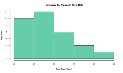
Quantitative data can be summarized using frequency distributions, histograms, and box plots.

Audit Time (days)	Frequency	Proportion	Percentage
10–15	6	0.30	30
16–20	7	0.35	35
21–25	4	0.20	20
26–30	2	0.10	10
31–35	1	0.05	5
Total	20	1.00	100

Box Plot

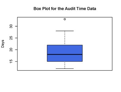
A box plot visually summarizes the distribution of data, showing the median, quartiles, and potential outliers.

• Box: Spans from Q1 (25th percentile) to Q3 (75th percentile).

• Line in box: Median value.

• Whiskers: Minimum and maximum values (excluding outliers).

• Outlier: Value outside the range Q1 - 1.5×IQR or Q3 + 1.5×IQR.

Numerical Measures of Location

• Mean (Sample Mean): $\bar{y} = \frac{1}{n} \sum_{i=1}^{n} y_i$

• Median: The middle value in an ordered dataset.

• Mode: The value that occurs most frequently.

• Percentiles: The value below which a given percentage of observations fall.

• Quartiles: Q1 (25th percentile), Q2 (median, 50th percentile), Q3 (75th percentile).

Numerical Measures of Variability (Dispersion)

• Range: Difference between maximum and minimum values.

• Variance (Sample): $S^2 = \frac{\sum_{i=1}^{n} (y_i - \bar{y})^2}{n-1}$

• Standard Deviation (Sample): $S = \sqrt{S^2}$

• Interquartile Range (IQR): $IQR = Q_3 - Q_1$

Mean vs. Median

• For symmetric distributions, mean = median.

• For skewed distributions, mean ≠ median (mean is pulled toward the longer tail).

Discussion: Statistical Thinking in Practice

Evaluating Statistical Claims

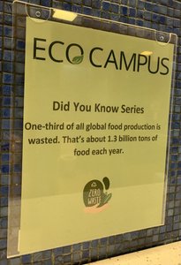
When encountering statistical statements (e.g., "One-third of all global food production is wasted. That’s about 1.3 billion tons of food each year."), consider:

• What is the population being studied?

• How is the key variable (e.g., "food waste") defined and measured?

• What data and methods support the estimate?

• What additional information would increase credibility?

Additional info: These foundational concepts prepare students for deeper topics such as probability, sampling, estimation, hypothesis testing, and regression analysis in business statistics.