 Back
BackHypothesis Testing for a Single Population: Comprehensive Study Notes
Study Guide - Smart Notes
 Tailored notes based on your materials, expanded with key definitions, examples, and context.
Chapter 9: Hypothesis Testing for a Single Population
9.1 An Introduction to Hypothesis Testing
Hypothesis testing is a fundamental statistical method used to make inferences about population parameters based on sample data. It involves formulating two competing hypotheses and using sample evidence to decide which is more plausible.
Hypothesis: An assumption about a population parameter (e.g., mean or proportion).
Null Hypothesis (H0): Represents the status quo or a specific value for the parameter. It is assumed true unless evidence suggests otherwise.
Alternative Hypothesis (H1): Represents a change or effect; the claim researchers often wish to support.
Types of Tests:
One-tail test: Tests for a parameter being greater than or less than a value.
Two-tail test: Tests for a parameter being different (not equal) to a value.
Example: Testing if the mean data use for smartphone users is μ = 1.8 GB/month.
Stating the Hypotheses
Formulate H0 and H1 based on the research question.
H0 typically uses ≤, =, or ≥; H1 uses >, ≠, or <.
The alternative hypothesis is also called the research hypothesis.
Examples of Hypothesis Pairs:
H0: μ ≥ 1.8, H1: μ < 1.8
H0: μ ≤ 1.8, H1: μ > 1.8
H0: μ = 1.8, H1: μ ≠ 1.8
Logic of Hypothesis Testing
We never "accept" H0; we either reject it or fail to reject it based on sample evidence.
Sample results may not perfectly reflect the population due to sampling error.
Type I and Type II Errors
Errors can occur in hypothesis testing due to the uncertainty inherent in sampling.
Type I Error (α): Rejecting H0 when it is true (false positive).
Type II Error (β): Failing to reject H0 when it is false (false negative).
α is the level of significance (probability of Type I error).
β is the probability of Type II error.
Reducing α increases β for a fixed sample size; increasing sample size reduces both.
Application Example: In quality control, Type I error is the producer’s risk, and Type II error is the consumer’s risk.
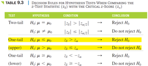
Decision Rules for Hypothesis Tests
Decision rules specify when to reject or not reject H0 based on the test statistic or p-value.
Test | Hypothesis | Condition | Conclusion |
|---|---|---|---|
Two-tail | H0: μ = μ0 | |zt| > |zα/2| | Reject H0 |
Two-tail | H0: μ = μ0 | |zt| ≤ |zα/2| | Do not reject H0 |
One-tail (upper) | H0: μ ≤ μ0 | zt > zα | Reject H0 |
One-tail (upper) | H0: μ ≤ μ0 | zt ≤ zα | Do not reject H0 |
One-tail (lower) | H0: μ ≥ μ0 | zt < -zα | Reject H0 |
One-tail (lower) | H0: μ ≥ μ0 | zt ≥ -zα | Do not reject H0 |
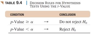
Decision Rules Using the p-Value
Condition | Conclusion |
|---|---|
p-value ≥ α | Do not reject H0 |
p-value < α | Reject H0 |
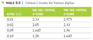
Critical z-Scores for Various Alphas
Alpha (α) | One Tail: Critical z-Score | Two Tail: Critical z-Score |
|---|---|---|
0.01 | 2.33 | 2.575 |
0.02 | 2.05 | 2.33 |
0.05 | 1.645 | 1.96 |
0.10 | 1.28 | 1.645 |
9.2 Hypothesis Testing for the Population Mean When σ Is Known
Assumptions and Steps
If n < 30, population must be normal; if n ≥ 30, Central Limit Theorem applies.
Use the z-test statistic when σ is known.
Formula for the z-test statistic:
\( \overline{x} \): sample mean
\( \mu_0 \): hypothesized population mean
\( \sigma \): population standard deviation
\( n \): sample size
Example: Testing if a new CFL bulb lasts more than 8,000 hours with n = 36, \( \overline{x} = 8,120 \), \( \sigma = 500 \), α = 0.05.
9.3 Hypothesis Testing for the Population Mean When σ Is Unknown
Student’s t-Distribution
When the population standard deviation is unknown, use the sample standard deviation (s) and the t-distribution.
Assume the population is normal.
Degrees of freedom = n – 1.
Formula for the t-test statistic:
\( s \): sample standard deviation
Example: Testing if the average hotel room cost in Chicago is less than $188, with n = 25, \( \overline{x} = 177.50 \), s = 25.40, α = 0.05.
Critical t-values can be found in statistical tables or using Excel functions (e.g., T.INV, T.INV.2T).
9.4 Hypothesis Testing for the Proportion of a Population
Testing Population Proportions
Used for hypotheses about population proportions (p).
Sample size must satisfy np ≥ 5 and n(1 – p) ≥ 5 for normal approximation.
Sample Proportion Formula:
\( x \): number of successes
\( n \): sample size
z-test Statistic for Proportion:
\( \hat{p} \): sample proportion
\( p_0 \): hypothesized population proportion
Example: Testing if the proportion of 4G contracts has increased from 0.62, with n = 350, x = 238, α = 0.05.
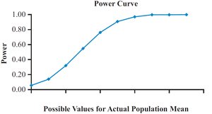
9.5 Type II Errors and Power of a Test
Type II Error (β) and Power
β is the probability of failing to reject a false null hypothesis.
Power of a test = 1 – β (probability of correctly rejecting H0).
As the true mean moves further from the hypothesized mean, power increases.
Increasing sample size reduces both α and β.
Calculating β for Population Means and Proportions
For means, calculate the probability of not rejecting H0 when the true mean differs from the hypothesized mean.
For proportions, use the critical sample proportion in place of the mean.
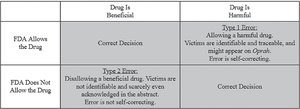
Special Application: FDA Drug Approval and Hypothesis Testing
The FDA’s drug approval process can be viewed as a hypothesis test:
H0: Drug has no effect or is harmful
H1: Drug is beneficial
Type I Error: Approving a harmful drug (false positive)
Type II Error: Not approving a beneficial drug (false negative)
Drug is Beneficial | Drug is Harmful | |
|---|---|---|
FDA Allows the Drug | Correct Decision | Type I Error: Allowing a harmful drug |
FDA Does Not Allow the Drug | Type II Error: Disallowing a beneficial drug | Correct Decision |
Appendix: Statistical Tables and Copyright Notice
Statistical tables (z and t) are essential for finding critical values in hypothesis testing. Always ensure proper use of copyrighted materials in academic settings.

Additional info: The above notes include expanded explanations, formulas, and context for all major topics in Chapter 9, suitable for business statistics students preparing for exams.
