One-Way ANOVA and Multiple Comparisons: Bonferroni and Tukey Methods

One-Way Analysis of Variance (ANOVA)

Introduction to One-Way ANOVA

One-way ANOVA is a statistical method used to test whether there are significant differences among the means of three or more independent groups. It is commonly applied in business statistics to compare group means in experiments or observational studies.

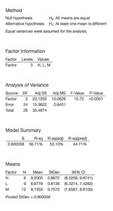
• Null Hypothesis (H0): All group means are equal.

• Alternative Hypothesis (Ha): At least one group mean is different.

• Assumptions: Independence, normality, and equal variances among groups.

Example Application: Comparing productivity improvements across firms with different R&D expenditure levels (low, moderate, high).

ANOVA Table and Interpretation

The ANOVA table summarizes the sources of variation, their degrees of freedom, sum of squares, mean squares, F-value, and p-value. A significant F-value (p < 0.05) indicates that not all means are equal.

Source	SS	DF	MS	F	P-value
Between Groups (e.g., R&D)	20.125	2	10.062	15.72	<0.0001
Error	15.362	24	0.6401
Total	35.487	26

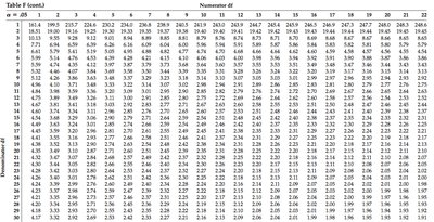
Interpretation: If the F-value is greater than the critical value from the F-distribution (e.g., 3.40 for df=2,24 at α=0.05), we reject H0 and conclude that at least one mean differs.

Multiple Comparisons and the Bonferroni Method

The Multiple Comparisons Problem

After finding a significant ANOVA result, the next step is to determine which means differ. Conducting multiple pairwise t-tests increases the risk of Type I error (false positives). This is known as the multiple comparisons problem.

• Type I Error Rate: Probability of incorrectly rejecting at least one true null hypothesis increases with the number of comparisons.

• Familywise Error Rate (FWER): The probability of making one or more Type I errors in a set (family) of comparisons.

Example: For 4 groups, there are 6 pairwise comparisons. Using a 95% confidence interval for each, the probability that at least one interval does not contain the true difference is approximately 26%.

Bonferroni Correction

The Bonferroni method adjusts the significance level to control the familywise error rate. For n comparisons and desired familywise significance level α, each test uses a significance level of α/n.

• Adjusted Confidence Level: $1 - \frac{\alpha}{n}$ for each interval.

• Adjusted t-value: Use the t-distribution with right-tail probability $\frac{\alpha}{2n}$ for two-sided intervals.

Formula for Bonferroni Confidence Interval:

$\left( \bar{x}_i - \bar{x}_j \right) \pm t^*_{\alpha/(2n),\,df} \cdot s_p \sqrt{\frac{1}{n_i} + \frac{1}{n_j}}$

• $\bar{x}_i, \bar{x}_j$ = sample means

• $s_p$ = pooled standard deviation

• $n_i, n_j$ = sample sizes

• $df$ = degrees of freedom (N - I)

Bonferroni Example: Productivity Improvements

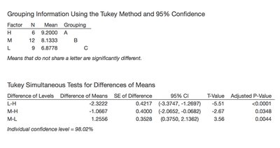
Suppose we compare productivity means for three R&D levels (Low, Moderate, High):

R&D Level	Mean	SD	n
Low	6.878	0.814	9
Moderate	8.133	0.757	12
High	9.200	0.867	6

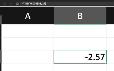
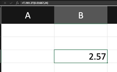
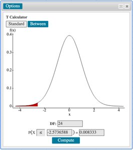
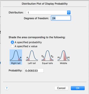
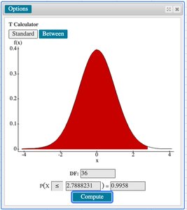
There are 3 comparisons. For a familywise confidence level of 0.95, each interval uses a confidence level of 0.9833. The critical t-value is found using statistical software (e.g., t = 2.57 for df = 24).

Conclusion: If zero is not in any confidence interval, we conclude all means differ significantly.

Tukey's Honestly Significant Difference (HSD) Method

Overview of Tukey's HSD

Tukey's HSD is another method for multiple comparisons that controls the familywise error rate and is especially useful for comparing all possible pairs of means after ANOVA.

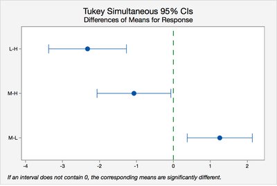
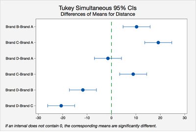
• Simultaneous Confidence Intervals: Tukey's method provides intervals for all pairwise differences.

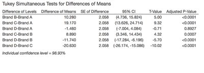
• Interpretation: If an interval does not contain zero, the corresponding means are significantly different.

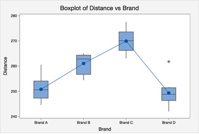
ANOVA and Multiple Comparisons: Golf Ball Example

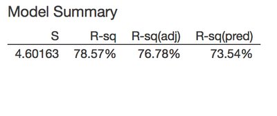
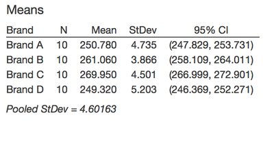
Data and Model Summary

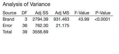
Suppose we compare the mean distance for four brands of golf balls. The ANOVA table and model summary are as follows:

Source	DF	Adj SS	Adj MS	F-Value	P-Value
Brand	3	2794.39	931.463	43.99	<0.0001
Error	36	762.30	21.175
Total	39	3556.69

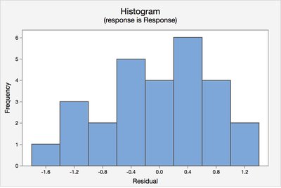
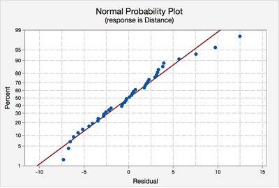
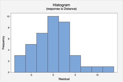
Checking ANOVA Assumptions

Normal probability plots and histograms of residuals are used to check the assumptions of normality and equal variance. Boxplots help identify outliers and skewness.

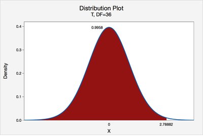
Bonferroni and Tukey Methods in Practice

For four brands, there are 6 pairwise comparisons. The Bonferroni-adjusted t-value is calculated using statistical software (e.g., t = 2.79 for df = 36). Tukey's method provides simultaneous confidence intervals for all pairs.

Summary Table: Bonferroni vs. Tukey Methods

Method	Purpose	Adjustment	When to Use
Bonferroni	Controls familywise error rate for any set of comparisons	Divides α by number of comparisons	Small number of planned comparisons
Tukey HSD	All pairwise comparisons after ANOVA	Uses studentized range distribution	All possible pairwise comparisons

Key Formulas

• ANOVA F-statistic: $F = \frac{MS_{Between}}{MS_{Within}}$

• Pooled Standard Deviation: $s_p = \sqrt{\frac{\sum_{i=1}^I (n_i - 1)s_i^2}{N - I}}$

• Bonferroni CI for difference of means: $\left( \bar{x}_i - \bar{x}_j \right) \pm t^*_{\alpha/(2n),\,df} \cdot s_p \sqrt{\frac{1}{n_i} + \frac{1}{n_j}}$

Conclusion

One-way ANOVA is a powerful tool for comparing means across multiple groups. When significant differences are found, multiple comparison procedures such as Bonferroni and Tukey's HSD are essential for identifying which means differ while controlling the overall error rate. Proper checking of assumptions and use of statistical software for critical values are important for valid inference.