Probability Distributions: Discrete and Continuous Random Variables

Continuous Probability Distributions

Definition and Example

Continuous probability distributions describe the probabilities of the possible values of a continuous random variable. For example, let X be the length of time between arrivals at a drive-in teller machine. The probability distribution of X can be represented graphically and mathematically.

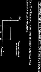
Functional Form of a Continuous Probability Distribution

The probability density function (pdf) for a continuous random variable X is defined as follows:

• f(x) = c for 5 < x < 15

• f(x) = 0 otherwise

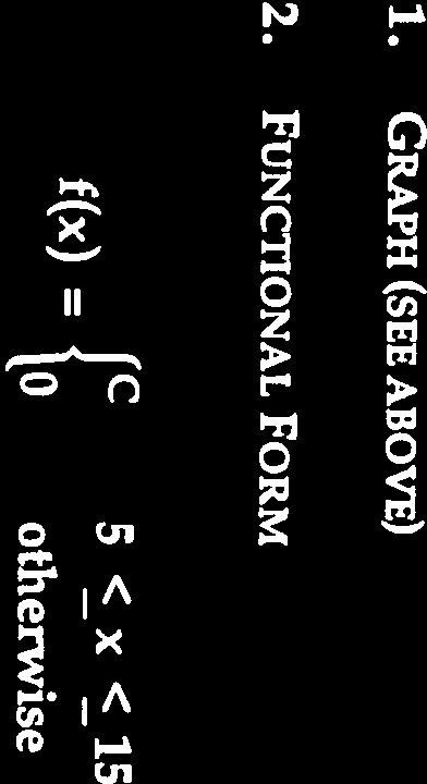
Here, c is a constant that ensures the total probability is 1.

Requirements for a Probability Density Function

For f(x) to be a valid probability distribution, the following must be true:

• f(x) ≥ 0 for all x

• The total area under the curve must equal 1: $\int_{-\infty}^{\infty} f(x) dx = 1$

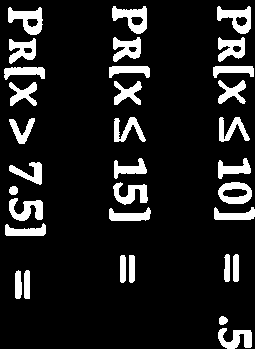
Calculating Probabilities for Continuous Random Variables

Probabilities for continuous random variables are calculated as the area under the probability density function between two points:

$\Pr[a \leq x \leq b] = \int_{a}^{b} f(x) dx$

For example, to find $\Pr[x \geq b]$, use:

$\Pr[x \geq b] = \int_{b}^{\infty} f(x) dx$

Uniform Distribution Example

For the uniform distribution defined above, the probability that X falls within a certain interval is proportional to the length of that interval. For example:

• $\Pr[x \leq 10] = 0.5$

• $\Pr[x \leq 15] = 1$

• $\Pr[x > 7.5] =$ (to be calculated)

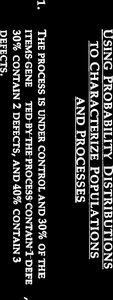
Using Probability Distributions to Characterize Populations and Processes

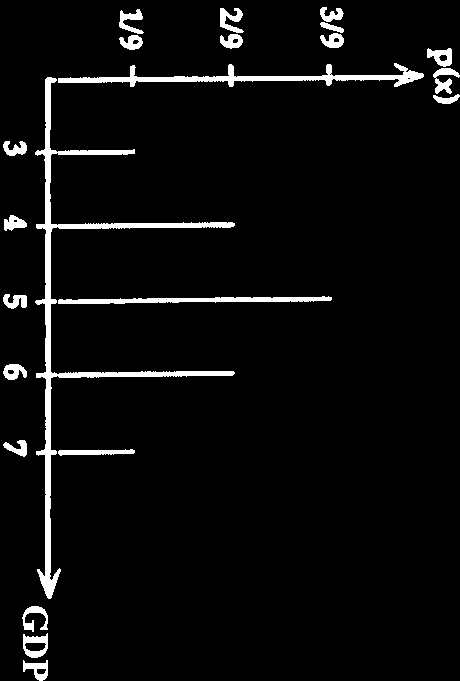
Discrete Probability Distributions

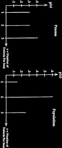
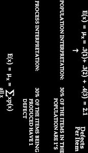
Discrete probability distributions describe the probability of each possible value of a discrete random variable. For example, consider a process where items can have 1, 2, or 3 defects with probabilities 0.3, 0.3, and 0.4, respectively.

Population and Process Interpretation

Suppose a production run generated 1000 items: 150 with 1 defect, 600 with 2 defects, and 250 with 3 defects. The probability distribution can be visualized as follows:

Mean (Expected Value) of a Probability Distribution

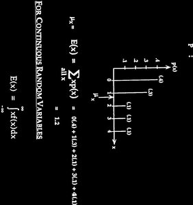
The mean or expected value of a probability distribution is a measure of central tendency. For a discrete random variable, it is calculated as:

$E(x) = \mu = \sum_{\text{all } x} x p(x)$

For a continuous random variable:

$E(x) = \int_{-\infty}^{\infty} x f(x) dx$

Variance and Standard Deviation of a Random Variable

The variance measures the spread of the distribution. For a discrete random variable:

$\sigma^2 = E[(x - \mu)^2] = \sum_{\text{all } x} (x - \mu)^2 p(x)$

For a continuous random variable:

$\sigma^2 = E[(x - \mu)^2] = \int_{-\infty}^{\infty} (x - \mu)^2 f(x) dx$

Special Probability Distributions

Uniform Distribution

The uniform distribution is a continuous probability distribution where all intervals of the same length within the distribution's range are equally probable. The pdf is:

$f(x) = \frac{1}{b-a}$ for $a \leq x \leq b$

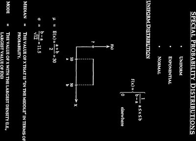
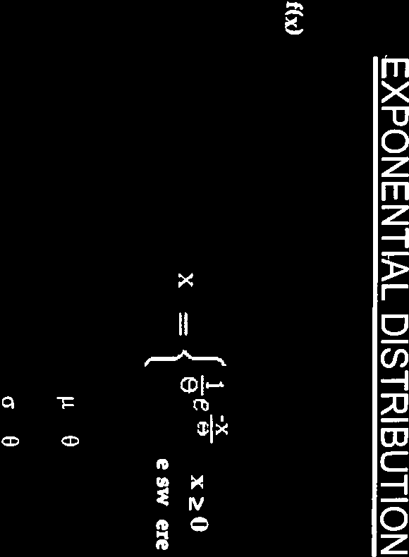
Exponential Distribution

The exponential distribution is used to model the time between events in a Poisson process. The pdf is:

$f(x) = \frac{1}{\theta} e^{-x/\theta}$ for $x \geq 0$

where $\theta$ is the mean (average time between arrivals).

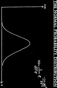
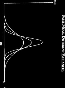
Normal Probability Distribution

The normal distribution is a continuous probability distribution characterized by its bell-shaped curve. The pdf is:

$f(x) = \frac{1}{\sqrt{2\pi}\sigma} e^{-\frac{(x-\mu)^2}{2\sigma^2}}$

Standard Normal Distribution and Z-Transformation

Any normal distribution can be transformed into the standard normal distribution (mean 0, standard deviation 1) using the Z-transformation:

$Z = \frac{X - \mu}{\sigma}$

Using the Normal Table

The normal table (Z-table) provides the area under the standard normal curve to the left of a given Z value. This area represents the probability that a standard normal random variable is less than or equal to Z.

Example: Calculating Probabilities with the Normal Distribution

Suppose the sales manager believes that next year's sales are normally distributed with mean 10,000 and standard deviation 2500. To find the probability that sales are less than or equal to 9000:

• Calculate Z: $Z = \frac{9000 - 10000}{2500} = -0.4$

• Look up the area for Z = -0.4 in the normal table: $P(Z \leq -0.4) = 0.3446$

Summary Table: Key Probability Distributions

Distribution	PDF	Mean	Variance
Uniform	$f(x) = \frac{1}{b-a}$ for $a \leq x \leq b$	$\frac{a+b}{2}$	$\frac{(b-a)^2}{12}$
Exponential	$f(x) = \frac{1}{\theta} e^{-x/\theta}$ for $x \geq 0$	$\theta$	$\theta^2$
Normal	$f(x) = \frac{1}{\sqrt{2\pi}\sigma} e^{-\frac{(x-\mu)^2}{2\sigma^2}}$	$\mu$	$\sigma^2$