Probability Distributions of Continuous Random Variables and the Normal Distribution

Probability Distributions of Continuous Random Variables

Introduction to Continuous Random Variables

Continuous random variables are variables that can take any value within a given interval, as opposed to discrete random variables which can only take specific values. These variables are fundamental in business statistics for modeling real-world phenomena such as time, mass, and distance.

• Random Variable (X): Associates a numerical value with each outcome of an experiment.

• Continuous Random Variable: Can take any value within an interval (e.g., time to complete a task, mass of luggage, daily distance traveled).

• Examples: The mass of a lion cub, delivery times, or electricity consumption.

Probability Distributions and Probability Density Function (PDF)

Continuous probability distributions are represented by curves, where the area under the curve between two values represents the probability that the variable falls within that interval. The probability density function (PDF) describes the distribution of probability for a continuous random variable.

• Properties of the PDF:

  • The total area under the curve is 1.

  • $P[a \leq X \leq b]$ is the area under the curve between $a$ and $b$.

  • $f(x) \geq 0$ for all $x$.

• Population Parameters: Mean ($\mu$), Variance ($\sigma^2$), and Standard Deviation ($\sigma$).

Conceptual Example: Mass of Lion Cubs

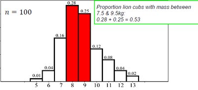
The mass of lion cubs can be modeled as a continuous random variable. Histograms and density curves are used to visualize the distribution of their masses.

• Relative Frequency Histogram: Shows the distribution of observed values in intervals.

• Probability Density Curve: Smooth curve representing the probability distribution.

The Normal Distribution

Definition and Properties

The normal distribution is the most widely used continuous probability distribution in practice. It is mathematically derived and is a good model for many natural and business phenomena. The normal distribution is symmetric about the mean and its shape is determined by the mean ($\mu$) and standard deviation ($\sigma$).

• Notation: $N(\mu, \sigma^2)$ denotes a normal distribution with mean $\mu$ and variance $\sigma^2$.

• Symmetry: The curve is symmetric with respect to the mean.

• Effect of Standard Deviation: Larger $\sigma$ results in a flatter curve; smaller $\sigma$ results in a steeper curve.

The Standard Normal Distribution

The standard normal distribution is a special case of the normal distribution with mean $0$and standard deviation $1$. The corresponding random variable is denoted by $Z$.

• Notation: $Z \sim N(0, 1)$

• Standardization: Any normal random variable $X$ can be transformed to $Z$ using the formula:

$Z = \frac{X - \mu}{\sigma}$

Calculating Probabilities Using the Standard Normal Table

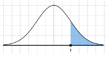
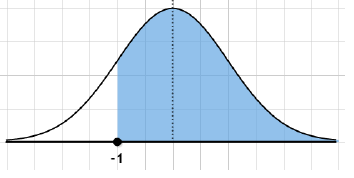
Probabilities for the standard normal distribution are found using the standard normal (Z) table, which gives the area to the left of a specified Z value. Probabilities for any normal random variable can be calculated by first converting to the standard normal variable.

• Key Properties:

  • $P[Z \leq 0] = 0.5$

  • $P[Z \leq -a] = 1 - P[Z \leq a] = P[Z \geq a]$

  • $P[Z > a] = 1 - P[Z \leq a]$

  • $P[a \leq Z \leq b] = P[Z \leq b] - P[Z \leq a]$

Examples of Probability Calculations

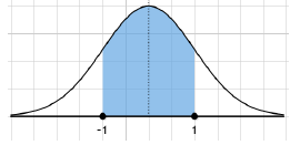
To calculate probabilities for a normal random variable $X$, first convert $X$ to $Z$ using the standardization formula, then use the Z-table to find the required probability.

• Example: Calculate $P(Z \leq 1)$, $P(Z > 0.43)$, $P(Z < -2.11)$, $P(-2.54 \leq Z \leq 1.83)$.

Finding Percentiles and X-Limits for Given Probabilities

Sometimes, the probability associated with an unknown $x$-value is given, and the task is to find the corresponding $x$-value. This involves reversing the standardization process:

1. Sketch the normal curve.

2. Use the Z-table to identify the Z-value that corresponds to the given area (probability).

3. Use the transformation $x = \mu + z\sigma$ to find the corresponding $x$-value.

Example: A marketing manager wants to find the minimum purchase value for the highest-spending 15% of customers. Find the $x$-value such that $P(X > x) = 0.15$.

Summary Table: Properties of the Normal Distribution

Property	Description
Mean ($\mu$)	Center of the distribution; location of symmetry
Standard Deviation ($\sigma$)	Controls the spread/width of the curve
Total Area	Equals 1 (represents total probability)
Symmetry	Curve is symmetric about the mean
Empirical Rule	~68% within 1$\sigma$, ~95% within 2$\sigma$, ~99.7% within 3$\sigma$

Additional info:

• The normal distribution is foundational for inferential statistics, including hypothesis testing and confidence intervals.

• The standard normal table (Z-table) is essential for finding probabilities and percentiles for normally distributed variables.