Random Variables and Probability Distributions: Study Notes

Random Variables and Probability Distributions

Introduction

This chapter introduces the concept of random variables, distinguishes between discrete and continuous types, and explores their probability distributions. Special focus is given to the binomial and normal distributions, which are foundational in business statistics.

4.1 Two Types of Random Variables

Definition of a Random Variable

A random variable is a variable that assumes numerical values associated with the random outcomes of an experiment, where one numerical value is assigned to each sample point. It is essentially a function that maps outcomes of a random process to numbers.

Discrete Random Variables

Discrete random variables can assume a countable number (finite or infinite) of values. Examples include the number of sales made in a week, the number of errors on a page, or the number of customers waiting in line.

• Examples:

  • Number of sales made by a salesperson in a week: x = 0, 1, 2, ...

  • Number of errors on a page: x = 0, 1, 2, ...

  • Number of visitors to a website in a day: x = 0, 1, 2, ...

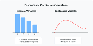
Continuous Random Variables

Continuous random variables can assume any value within a given interval or range. These variables are measured, not counted, and can take on infinitely many possible values.

• Examples:

  • Weight of a T-bone steak

  • Time taken to complete a task

  • Length of time between phone charges

Practice: Classification

• Weight of T-bone steak: Continuous

• Exact time to evaluate 27 + 72: Continuous

• Number of textbook authors at a computer: Discrete

• Number of statistics students reading a book: Discrete

• Number of website visitors in a day: Discrete

4.2 Probability Distributions for Discrete Random Variables

Discrete Probability Distribution

A probability distribution for a discrete random variable is a graph, table, or formula that specifies the probability associated with each possible value the random variable can assume. This is also called a probability mass function (PMF).

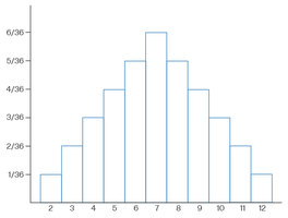
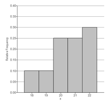
Graphical and Tabular Representations

Probability distributions can be represented as bar graphs or tables, showing the probability for each value of the random variable.

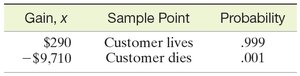
Example: Insurance Application

Suppose an insurance company sells a $10,000 one-year term insurance policy at an annual premium of $290. The probability of death during the next year is 0.001. The expected gain for the company can be calculated using the probability distribution:

Gain, x	Sample Point	Probability
$290	Customer lives	0.999
-$9,710	Customer dies	0.001

4.3 The Binomial Distribution

Definition and Characteristics

The binomial distribution models the number of successes in a fixed number of independent trials, each with the same probability of success. It is used for experiments with dichotomous outcomes (e.g., success/failure, yes/no).

• The experiment consists of n identical trials.

• Each trial has two possible outcomes: Success (S) or Failure (F).

• The probability of success (p) is constant for each trial; probability of failure is q = 1 - p.

• Trials are independent.

• The binomial random variable x is the number of successes in n trials.

Binomial Probability Formula

The probability of observing exactly x successes in n trials is given by:

$P(X = x) = \binom{n}{x} p^x q^{n-x}$

where $\binom{n}{x}$ is the binomial coefficient, p is the probability of success, and q is the probability of failure.

Example: Manufacturing

A machine produces 10% defectives. If the next five items are tested, the probability that three are defective is found using the binomial formula with n = 5, p = 0.1, q = 0.9.

4.5 Probability Distributions for Continuous Random Variables

Continuous Probability Density Function (PDF)

The probability distribution for a continuous random variable is described by a probability density function (PDF), which is a smooth curve. The probability that the variable falls within a certain interval is given by the area under the curve over that interval.

Conditions for a PDF

• f(x) ≥ 0 for all x

• The total area under the curve is 1: $\int_{-\infty}^{\infty} f(x) dx = 1$

Finding Probability

The probability that a continuous random variable x falls between a and b is:

$P(a \leq x \leq b) = \int_{a}^{b} f(x) dx$

4.6 The Normal Distribution

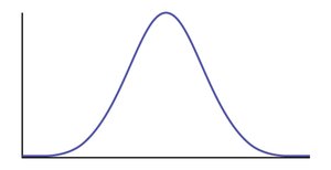
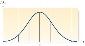
Definition and Properties

The normal distribution is a continuous probability distribution that is bell-shaped and symmetric about the mean. The mean, median, and mode are all equal. The normal distribution is fundamental in statistics due to the Central Limit Theorem.

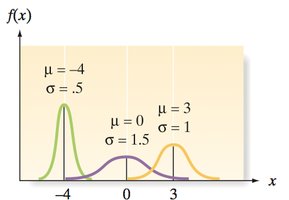
Effect of Different Means and Standard Deviations

Normal distributions can have different means (μ) and standard deviations (σ), which affect the center and spread of the curve, respectively.

Standard Normal Distribution

The standard normal distribution is a special case with mean μ = 0 and standard deviation σ = 1. Probabilities are found using the standard normal (z) table.

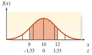
Converting Normal to Standard Normal

Any normal random variable x with mean μ and standard deviation σ can be converted to a standard normal variable z using:

$z = \frac{x - \mu}{\sigma}$

Finding Probabilities Using the z-Table

To find the probability that x falls within a certain range, convert the x-values to z-scores and use the z-table to find the corresponding area under the curve.

Example: Cell Phone Application

Suppose the time between charges for a cell phone is normally distributed with mean 10 hours and standard deviation 1.5 hours. To find the probability that the phone lasts between 8 and 12 hours, convert 8 and 12 to z-scores and find the area between them.

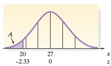
Example: Advertised Gas Mileage

An automobile has a mean in-city mileage of 27 mpg (σ = 3 mpg). To find the probability that a car gets less than 20 mpg, calculate the z-score for 20 and find the area to the left of this value.

Percentiles and Incentives

Percentiles in a normal distribution can be used for decision-making, such as setting incentive bonuses for production exceeding a certain threshold (e.g., the 90th percentile).

Additional info: These notes include expanded definitions, formulas, and examples to ensure a comprehensive understanding of random variables and probability distributions, as required for business statistics students.