Sampling and Sampling Distributions: Core Concepts and Applications

Sampling and Sampling Distributions

7.1 Why Sample?

Sampling is a fundamental process in statistics, allowing researchers to draw conclusions about a population by examining a subset of its members. This approach is essential when it is impractical or impossible to measure the entire population.

• Population: The entire group of subjects of interest.

• Sample: A subset of the population, selected for analysis.

• Purpose of Sampling: To make accurate inferences about the population while saving time and resources.

7.2 Types of Sampling and Biases

There are several methods for selecting samples, each with its own advantages and limitations. Proper sampling methods reduce bias and improve the reliability of statistical inferences.

Probability Sampling

• Probability Sample: Each member of the population has a known, nonzero chance of being selected. Enables inferential statistics.

Simple Random Sampling

• Every member has an equal chance of selection.

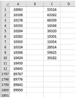
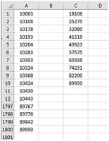
• Often implemented using random number generators or software tools like Excel.

Systematic Sampling

• Every kth member is chosen, where k = N/n (N = population size, n = sample size).

• Easy to implement but may be affected by periodicity in the population.

Stratified Sampling

• Population is divided into strata (homogeneous groups), and random samples are drawn from each stratum.

• Ensures representation of key subgroups.

Cluster Sampling

• Population is divided into clusters (often geographically), and entire clusters are randomly selected.

• Clusters are heterogeneous mini-populations.

Resampling

• Statistical technique involving repeated sampling from the available data (e.g., bootstrap method).

Nonprobability Sampling

• Probability of selection is unknown (e.g., convenience sampling).

• Quick and easy but may not be representative.

Biases in Sampling

• Sampling Bias: Sample is not representative of the population.

• Nonresponse Bias: Differences between respondents and nonrespondents.

• Response Bias: Inaccurate answers due to question wording or respondent behavior.

• Undercoverage Bias: Some population segments are inadequately represented.

• Voluntary Response Bias: Those who volunteer differ systematically from those who do not.

• Cognitive Biases: Logical errors in reasoning (anchoring, availability heuristic, confirmation, recency).

7.3 Sampling and Nonsampling Errors

Errors can arise from both the sampling process and other aspects of data collection.

• Parameter: Value describing a population characteristic (e.g., mean, median).

• Statistic: Value calculated from a sample.

• Sampling Error: Difference between a sample statistic and the corresponding population parameter.

Formula for Sampling Error of the Sample Mean:

$\text{Sampling Error} = \overline{x} - \mu$

• Nonsampling Errors: Errors not related to sampling variability (e.g., ambiguous questions, data collection mistakes).

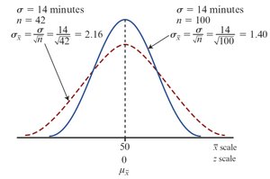
7.4 The Central Limit Theorem (CLT)

The Central Limit Theorem is a cornerstone of inferential statistics. It states that the distribution of sample means approaches normality as the sample size increases, regardless of the population's distribution.

• For large samples (n ≥ 30), the sampling distribution of the mean is approximately normal.

• If the population is normal, the sampling distribution is normal for any sample size.

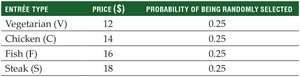
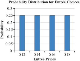
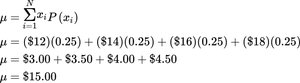
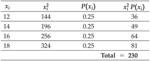
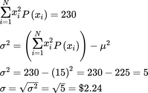
Population Example: Entrée Prices

Entrée Type	Price ($)	Probability
Vegetarian (V)	12	0.25
Chicken (C)	14	0.25
Fish (F)	16	0.25
Steak (S)	18	0.25

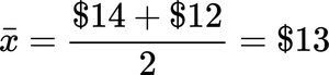
Population Mean Calculation:

Population Standard Deviation Calculation:

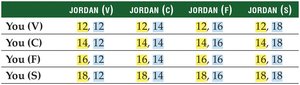
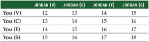
Sampling Distribution Example

All possible pairs of entrée choices (n = 2) are listed, and their averages are calculated to form the sampling distribution of the mean.

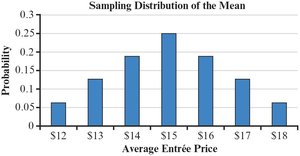
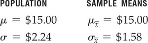
Key Properties of the Sampling Distribution of the Mean

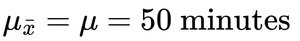
• The mean of the sampling distribution equals the population mean: $\mu_{\overline{x}} = \mu$

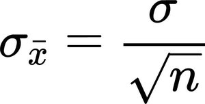
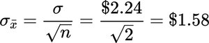
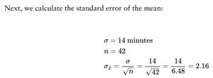
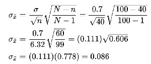
• The standard deviation of the sampling distribution (standard error): $\sigma_{\overline{x}} = \frac{\sigma}{\sqrt{n}}$

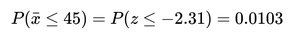
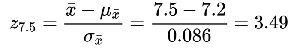
Application: Testing Claims Using the CLT

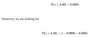
To test claims about population means, calculate the probability of observing a sample mean as extreme as the one obtained, assuming the null hypothesis is true.

• Calculate the standard error of the mean.

• Compute the z-score for the observed sample mean.

• Find the probability using the standard normal distribution.

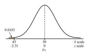
The Effect of Sample Size

• As sample size increases, the standard error decreases, making the sampling distribution narrower and reducing sampling error.

Finite Population Correction

When the sample size is more than 5% of the population, adjust the standard error using the finite population correction factor:

$\sigma_{\overline{x}} = \frac{\sigma}{\sqrt{n}} \sqrt{\frac{N-n}{N-1}}$

7.5 The Sampling Distribution of the Proportion

When dealing with proportions, the sampling distribution describes the pattern of sample proportions from repeated random samples.

• Underlying distribution is binomial.

• Conditions: $np \geq 5$ and $nq \geq 5$ (where $q = 1 - p$).

Sample Proportion Formula:

$\overline{p} = \frac{x}{n}$

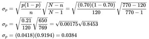
Standard Error of the Proportion:

$\sigma_{p} = \sqrt{\frac{p(1-p)}{n}} \sqrt{\frac{N-n}{N-1}}$

Z-score for the Sample Proportion:

$z = \frac{\overline{p} - p}{\sigma_{p}}$

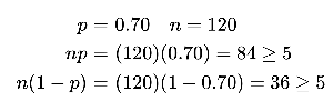
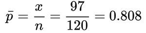
Example: Testing a Proportion Claim

• Population: 770 students, claimed proportion $p = 0.70$.

• Sample: 120 students, 97 successes ($\overline{p} = 0.808$).

• Check conditions: $np = 84 \geq 5$, $nq = 36 \geq 5$.

• Calculate standard error and z-score.

• Find probability and draw conclusion.

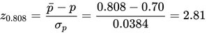
Conclusion

If the probability of observing the sample proportion (or more extreme) is very small under the null hypothesis, we have evidence to suggest the population proportion is different from the claimed value.

Additional info: These notes provide a comprehensive overview of sampling methods, errors, the Central Limit Theorem, and the sampling distributions of means and proportions, with practical examples and relevant formulas for business statistics students.