week 1-1 ch 10

Chapter 10: Sampling Distributions

Introduction to Sampling Distributions

Sampling distributions are fundamental in statistics, especially for making inferences about populations based on sample data. This chapter explores how sample statistics, such as proportions and means, vary from sample to sample and how these variations can be modeled mathematically.

• Sampling Distribution: The probability distribution of a given statistic based on a random sample.

• Importance: Allows estimation of population parameters and quantification of sampling variability.

Learning Objectives

• Understand how variations among multiple samples are represented in a sampling distribution.

• Calculate the mean and variance of the sampling distribution for proportions and means.

• Apply these concepts to estimate population characteristics.

10.1 Modelling Sample Proportions

Understanding Sample Proportions

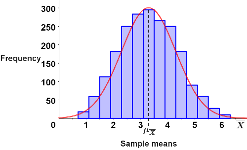
When repeatedly sampling from a population, the proportion of successes in each sample (denoted as p-hat, or \( \hat{p} \)) will vary. The distribution of these sample proportions forms the sampling distribution of the proportion.

• Example: Drawing 1000 samples of size 100 from a population where 20% are under 15 years old (\( p = 0.2 \)).

• Each sample yields a value of \( \hat{p} \), and the collection of these values forms a distribution.

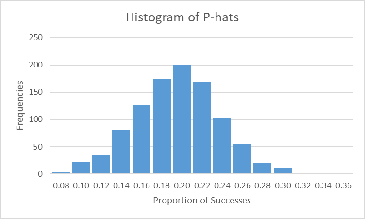
Interpretation: The histogram above shows the variability of sample proportions around the true population proportion.

Mean and Standard Deviation of Sample Proportions

• Mean of \( \hat{p} \): The average of all sample proportions equals the true population proportion \( p \).

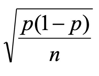
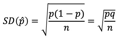
• Standard Deviation of \( \hat{p} \): Measures the spread of sample proportions around the mean.

The formulas are:

• Mean: $\mu_{\hat{p}} = p$

• Standard Deviation: $\sigma_{\hat{p}} = \sqrt{\frac{p(1-p)}{n}}$

Conditions for Normal Approximation

• Sample size must be large enough: $np > 10$ and $n(1-p) > 10$

• Samples must be independent and randomly selected.

• If sampling without replacement, $n < 0.1N$ (10% condition).

10.2 The Sampling Distribution for Proportions

Definition and Properties

The sampling distribution of the proportion is the distribution of sample proportions over many independent samples from the same population. It is typically bell-shaped and centered at the true proportion \( p \).

• Standard deviation: $SD_{\hat{p}} = \sqrt{\frac{pq}{n}}$ where $q = 1 - p$

• Sampling error: The difference between a sample proportion and the true population proportion, reflecting expected variability.

Assumptions and Conditions

• Independence Assumption: Sampled values must be independent.

• Sample Size Assumption: Sample size must be large enough for the normal approximation to hold.

• Randomization Condition: Data must be randomly sampled or randomly assigned.

• 10% Condition: Sample size should be no more than 10% of the population if sampling without replacement.

• Success/Failure Condition: Both $np$ and $nq$ should be at least 10.

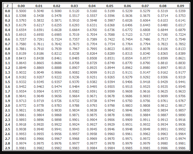
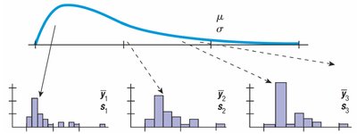
10.3 The Central Limit Theorem (CLT)

Statement and Importance

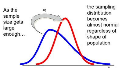
The Central Limit Theorem (CLT) is a cornerstone of statistics. It states that the sampling distribution of the sample mean (or proportion) approaches a normal distribution as the sample size increases, regardless of the population's original distribution.

• Key Point: The larger the sample size, the better the normal approximation.

• Application: Allows use of normal probability models for inference even when the population is not normal.

Sample vs. Sampling Distribution

• Distribution of a sample: The pattern of values in a single sample, which may not be normal.

• Sampling distribution: The distribution of a statistic (mean or proportion) over many samples, which becomes normal as sample size increases.

10.4 The Sampling Distribution of the Mean

Standard Deviation of the Sample Mean

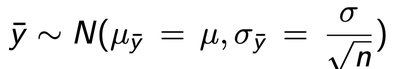
For a population with mean \( \mu \) and standard deviation \( \sigma \), the sampling distribution of the sample mean \( \bar{y} \) is:

• Mean: $\mu_{\bar{y}} = \mu$

• Standard deviation: $\sigma_{\bar{y}} = \frac{\sigma}{\sqrt{n}}$

Cases for Sampling Distribution of the Mean

• Case 1: Population normal, \( \sigma \) known: $\bar{y} \sim N(\mu, \frac{\sigma}{\sqrt{n}})$

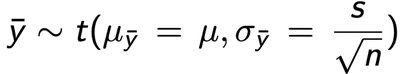
• Case 2: Population normal, \( \sigma \) unknown: $\bar{y} \sim t(\mu, \frac{s}{\sqrt{n}})$ with $n-1$ degrees of freedom

• Case 3: Population not normal, \( \sigma \) known: $\bar{y} \sim N(\mu, \frac{\sigma}{\sqrt{n}})$ if $n$ is large enough (CLT applies)

Assumptions and Conditions for Means

• Independence assumption

• Randomization condition

• 10% condition

• Large enough sample condition (especially for skewed populations)

Example: Probability Calculation for Sample Mean

Suppose box weights are unimodal and symmetric with mean 12 kg and standard deviation 4 kg. For a pallet of 10 boxes, what is the probability the total weight exceeds 150 kg?

• Convert to mean: $150/10 = 15$ kg

• Standard deviation of mean: $SD_{\bar{Y}} = \frac{4}{\sqrt{10}} = 1.26$

• Find $P(\bar{Y} > 15)$ using the normal distribution:

$Z = \frac{15 - 12}{1.26} = 2.38$

Probability: $P(Z > 2.38) = 1 - 0.9913 = 0.0087$

10.5 Standard Error

Definition and Application

When the population standard deviation or proportion is unknown, we estimate the standard deviation of the sampling distribution using sample data. This estimate is called the standard error (SE).

• For sample proportion: $SE_{\hat{p}} = \sqrt{\frac{\hat{p}\hat{q}}{n}}$

• For sample mean: $SE_{\bar{y}} = \frac{s}{\sqrt{n}}$ where $s$ is the sample standard deviation.

Chapter 10 Review and Visual Summary

Connecting Concepts

Sampling distributions allow us to relate population parameters to sample statistics. The Central Limit Theorem justifies the use of normal models for inference, and standard errors provide practical estimates when population parameters are unknown.

10.6 Common Pitfalls

• Do not confuse the sampling distribution with the distribution of a single sample.

• Ensure independence and randomization in sampling.

• Be cautious with small samples, especially for proportions and skewed populations.

Summary Table: Key Formulas

Statistic	Mean	Standard Deviation / Standard Error
Sample Proportion (\( \hat{p} \))	$p$	$\sqrt{\frac{p(1-p)}{n}}$ or $\sqrt{\frac{\hat{p}\hat{q}}{n}}$
Sample Mean (\( \bar{y} \))	$\mu$	$\frac{\sigma}{\sqrt{n}}$ or $\frac{s}{\sqrt{n}}$